Chapter 1: Introduction

CHAPTER 1: Introduction.

IBM said "It was to have been the nuclear age, it became the computer age..." The computer is now an indispensable tool in power system operation and planning. We can find numerous literature/algorithms on loadflow, fault calculation, dynamic and transient analysis, relay coordination, state estimation, optimal dispatch, security analysis, network reduction, shunt Mvar optimization and others. All these studies are implemented on a computer and most of them requires loadflow as part of the software.

Loadflow or powerflow is a steady state or static solution of a power system given the set of conditions. The primary information derived from such calculation are the voltage angle and power flows. For offline applications, only the peak and off-peak conditions are of primary interest.For real time application, loadflow may be run every 5 minutes together with economic dispatching, state estimation, security analysis. We can find these softwares in a computerised energy control center.

There are myriad possible conditions of a power system. Consideration of such selection must be based on:

1. How should the total system demand be shared by on-line plants for economic operation? 2. Transmission lines and transformers have thermal ratings.How should the system demand and generation be distributed without overloading them? System stability should be maintained. 3. How should we schedule Mvar generation, Mvar capacitor/reactor, synchronous condensers, transformer taps so that there will be no undervoltage or overvoltage to critical busses? 4. If the power system is a part of a larger pool, it must maintain power scheduling commitments via its tie lines to neighboring system. How should the system generation be scheduled (hourly, every minute, AGC) so that its import-export be realized? 5. How should we expand our power system? What will happen 1,2,5,10,20 years from now? Where will the generating plants be constructed? What will be the transmission line configuration? Voltage level? Wire size? 6. Which transmission lines, transformers are critical to the system? Critical means that if that equipment is non operational, how much MW load should be out of power to have the system in a normal running mode, without overloads.

All these conditions can be answered only by running a loadflow program.

Definition of a Loadflow Problem

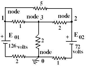
Loadflow or powerflow is a computer algorithm that displays the MW and MVAR loading of transmission lines and transformers after an iterative process of solving for node voltages. It is like using your ammeter and voltmeter and determine the junction voltages and current on the resistors of Figure 1. But instead of amperes, line flows are in MW and MVAR. Instead of E=126 volts from dry cells, the source feeding the circuit is in MW and MVAR. All other units are in per unit. Most chosen base MVA is 100.

Types of variables used

1. Uncontrollable or disturbance variable--Pd,Qd (demand)are beyond control since they are dictated by the customer. 2. State or dependent variable--Voltage magnitude and angle are computed based on the other two variables. 3. Control or independent variable--Has direct effect on the state variable. Mvar generation (Qg) greatly affects voltage magnitude. Mw generation (Pg) greatly affects voltage angle.

Classification of loadflow busses.

Type Known variables unknown variables
1. SL, Swing or Slack or Reference bus V,theta Pg,Qg
2. PV, Voltage controlled bus Pg,V Qg, theta
3. PQ, Load bus Pg, Qg, Pd, Qd V, theta

V- voltage magnitude
theta- voltage angle
Pg, Qg- Mw, Mvar generation
Pd, Qd- Mw, Mvar demand

Node Equations

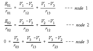
GSLF_Fig 1 Let us derive the nodal equation using a simple electrical circuit. The junctions formed when two or more elements (R, L, C ,etc)are connected are called nodes. One of them is designated as the Reference. By applying Kirchoff's current law, we can derive the nodal equations. The sum of current entering the node equals the sum of currents leaving the node. When making the current equation for node i, we assume that node to be of a higher potential than node j. In node 1 for example, the left side is the current source and the right side is [V(1)-V(2)]/r(1,2) + etc. Here node 1 is of a higher potential than node 2. We do this to all nodes except the reference. If there is no current source, put zero on the left side, as in node 3.

GSLF_Eq. 1
GSLF_Eq. 2
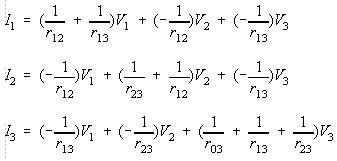
In Eq. (3), current sources is replaced by I. This is so because in power system analysis, current source is no longer a "cell" or a battery symbol with an "r" in series with that cell. Current source is a MW and MVAR generation and resistance in ohms as load is replaced by MW and MVAR demand or load. Connections between generator and load are transmission lines and transformers. These are in impedance in complex numbers with line charging in MVAR which are represented by pi equivalent.
Rearranging Eq. (2) in matrix form,
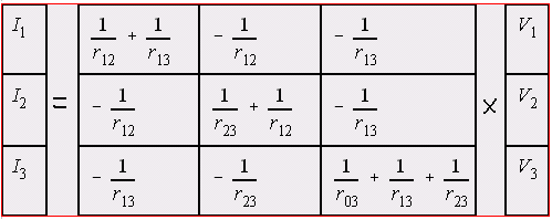GSLF_Eq. 3
The square matrix when replaced with line/transformer impedances becomes the bus admittance matrix or Ybus. The topic on Ybus formation is thoroughly discussed with examples on Chapter 5 of Part 1- Short Circuit Calculation.
In general, the diagonal part of the Ybus, Yii for node i is the sum of the admittances of all elements connected to node i. This may include connectiions to ground such as line charging, reactor/capacitor and the equivalent inductance for off-nominal transformers. Yij, (one of the off-diagonal element of the Ybus), is the negative of the admittance between node i and node j.

GSLF_Fig 2

Fig. (2) shows the direction of current flow. You will note that it obeys the Kirchoff's current law, "the algebraic sum of currents on each node is zero."

Shown on the text area below is a small program to compute for the matrix and solve the simultaneous linear equations using Gauss-Jordan Reduction. The input/output is also included. Numbers on the left are for purposes of discussion. Just copy, paste and delete the numbering if you need to compile it.

Program Listing_1: DC CIRCUIT FLOW

1: /* Program  DCFLOW, a loadflow like solution using
   2:    NODAL method with dc sources and resistance.
   3:    Solution of simultaneous linear equations by Gauss-Jordan Reduction  
   4:    contiguous bus numbering
   5:    
   6:    Date: October 5, 1999  Vancouver,BC, Canada
   7:    file: dcflow.cpp
   8:    Sparsity Technology, Joesel Pante
   9:    
  10: */
  11: #define LMAX 10
  12: #define BMAX  6
  13: #include <stdio.h>
  14: 
  15: int  np[LMAX], nq[LMAX],nl,nb;      
  16: //np[]=from bus, nq[]=to bus
  17: float r[LMAX],current[LMAX],E[LMAX];  
  18: //E[] input branch voltage , r[]=branch resistance, current[]=branch currents   
  19: float A[BMAX][BMAX+1],X[BMAX],B[BMAX];  
  20: //A[] -stores Ybus matrix, X[], B[]  in A.x=b
  21: FILE *file;
  22: 
  23: void Enter(void)
  24: {char *ch; printf("Enter to continue\n");gets(ch);}
  25:           
  26: 
  27: void input(void)
  28: { int k,m,i;     
  29:   float y;     
  30:   nb=0,nl=0; //initialize counters nl=lines, nb=bus 
  31:   for (i=0;i<BMAX;i++) 
  32:    {A[i][i]=(float)0.0;  //initialize diagonal part 
  33:     B[i]=(float)0.0;     //current sources, for multiple E source
  34:    } 
  35:   printf(" count  p   q   r_ohms  E_volts\n");
  36:   while (1)
  37:    { nl++; 
  38:      fscanf(file,"%d %d %f %f",np+nl,nq+nl,r+nl,E+nl);
  39:      if (np[nl]==99) break;
  40:      printf("%5d %3d %3d %7.2f %7.2f\n",
  41:          nl,np[nl],nq[nl],r[nl],E[nl]);
  42:      if (np[nl]>nb) nb=np[nl]; if (nq[nl]>nb) nb=nq[nl];  /*get the largest bus*/    
  43:      k=np[nl];m=nq[nl];  
  44: //in C or BASIC, k or m as zero has a place in the matrix. 
  45:      y=1/r[nl];
  46:      A[k][k]+=y;A[m][m]+=y; //the diagonal part   
  47:      A[k][m]=-y;A[m][k]=-y; //off-diagonal part    
  48:      B[m]+=E[nl]*y;  //based on input data, towards m is a positive Esource
  49:      B[k]-=E[nl]*y;
  50:     }
  51:    nl--;     //correct nl=lines read  
  52:    printf("number of lines:%2d  number of nodes:%2d\n",nl,nb);  
  53: //transfer b of A.x=b as augmented A
  54:   for (i=1; i<=nb; i++) A[i][nb+1]=B[i];   
  55: }
  56:  
  57:  
  58: void print(int size)  
  59: {int i,j;   
  60:  for (i=1;i<=size+1;i++) 
  61:    printf("%9d",i);printf("\n");  
  62:  for (i=1;i<=size;i++)
  63:    {printf("%2d ", i);  
  64:     for (j=1;j<=size+1;j++)
  65:      printf("%9.4f",A[i][j]); 
  66:     printf("\n");  
  67:    }  
  68:  printf("\n");
  69:  Enter();
  70: }
  71:  
  72: void gaussj()
  73: {int i1,j,k; 
  74:  float a1;
  75:  for (i1=1;i1<=nb;i1++)
  76:   {printf("for loop=%2d\n",i1);
  77:    a1=A[i1][i1];
  78:    for (j=i1;j<=nb+1; j++) A[i1][j]/=a1;
  79:    printf("After row is normalized\n"); print(nb);
  80:    for (j=1;j<=nb;j++)
  81:     {if (j!=i1)
  82:       {a1=A[j][i1];
  83:        for (k=i1;k<=nb+1;k++)
  84:          A[j][k]-=a1*A[i1][k];
  85:       }
  86:     }
  87:    printf("After Elimination\n"); print(nb);
  88:   }      
  89: }    
  90: 
  91: void flow(void)
  92: {int i,k,m;
  93:  printf("Node Voltage \n");
  94:  for (i=1;i<=nb;i++)
  95:   printf("%2d %8.2f\n",i,X[i]); 
  96:   
  97:  printf("Resulting branch flow\n"); 
  98:  printf("From  To  Current\n");  
  99:  for (i=1;i<=nl;i++)
 100:   {k=np[i];m=nq[i];//m is of a higher potential. Trace m to k.
 101:    current[i]=(X[m]-X[k]-E[i])/r[i]; 
 102:    printf("%5d %5d %8.2f\n",k,m,current[i]);
 103:   }     
 104: /*Output interpretation:
 105:  k, m entry  
 106:  flow away from a node is +
 107:  flow towards a node is -
 108:  
 109:  when m is of a higher potential than k
 110:  positive flow is m-->k
 111:  To trace back flow from k-->, negate it.
 112: */  
 113:  }
 114: 
 115:      
 116: void main(void)
 117: {int i;
 118:  file=fopen("dcflow.dat","r");
 119:  input(); 
 120:  printf("matrix printing A.x=b   A:b\n"); 
 121:  print(nb); 
 122:  printf("performing Gauss-Jordan Reduction\n"); 
 123:  gaussj();  //solve A.x=b where A is augmented with b
 124: //transfer the resulting x
 125:  for (i=1;i<=nb;i++) X[i]=A[i][nb+1];
 126: //solve branch currents  
 127:  flow(); 
 128:  i=flose(file);
 129: }

INPUT:
0  1  2  126
0  2  1   72
0  3  2   0
1  2  5   0
1  3  1   0
2  3  2   0
99 0 0 0

OUTPUT:
 count  p   q   r_ohms  E_volts
    1   0   1    2.00  126.00
    2   0   2    1.00   72.00
    3   0   3    2.00    0.00
    4   1   2    5.00    0.00
    5   1   3    1.00    0.00
    6   2   3    2.00    0.00
number of lines: 6  number of nodes: 3

matrix printing A.x=b   A:b
        1        2        3        4
 1    1.7000  -0.2000  -1.0000  63.0000
 2   -0.2000   1.7000  -0.5000  72.0000
 3   -1.0000  -0.5000   2.0000   0.0000
 
performing Gauss-Jordan Reduction
for loop= 1
After row is normalized
        1        2        3        4
 1    1.0000  -0.1176  -0.5882  37.0588
 2   -0.2000   1.7000  -0.5000  72.0000
 3   -1.0000  -0.5000   2.0000   0.0000

After Elimination
        1        2        3        4
 1    1.0000  -0.1176  -0.5882  37.0588
 2    0.0000   1.6765  -0.6176  79.4118
 3    0.0000  -0.6176   1.4118  37.0588

for loop= 2
After row is normalized
        1        2        3        4
 1    1.0000  -0.1176  -0.5882  37.0588
 2    0.0000   1.0000  -0.3684  47.3684
 3    0.0000  -0.6176   1.4118  37.0588

After Elimination
        1        2        3        4
 1    1.0000   0.0000  -0.6316  42.6316
 2    0.0000   1.0000  -0.3684  47.3684
 3    0.0000   0.0000   1.1842  66.3158

for loop= 3
After row is normalized
        1        2        3        4
 1    1.0000   0.0000  -0.6316  42.6316
 2    0.0000   1.0000  -0.3684  47.3684
 3    0.0000   0.0000   1.0000  56.0000

After Elimination
        1        2        3        4
 1    1.0000   0.0000   0.0000  78.0000
 2    0.0000   1.0000   0.0000  68.0000
 3    0.0000   0.0000   1.0000  56.0000

Node Voltage 
 1    78.00
 2    68.00
 3    56.00

Resulting branch flow
From  To  Current
    0     1   -24.00
    0     2    -4.00
    0     3    28.00
    1     2    -2.00
    1     3   -22.00
    2     3    -6.00

Code Explanation:
In Gauss-Jordan reduction, the matrix A is augmented by the vector b (in A.x=b). The objective is to make A a unity matrix by normalizing each row and elimination the upper and lower A(i,j) for each diagonal of node i. Each process of the normalizing and elimination is depicted in the output. There are only 3 major subroutines, input(), gaussj() and flow(). Subroutine input() reads the data and rightaway forms the Ybus.

i n n o v a t e o r s t a g n a t e