3.1 Triangularization of a Matrix
This chapter is taken from "Book 1: Short Circuit Calculation", modified and topics on Forward and Backward Course were included to suit the subject on Loadflow.
Triangularization is the process of applying Gauss-Jordan Reduction to solve the simultaneous linear equation of the form Ax=b. LU Factorization where L="Lower" and U="Upper" is synonymous to triangularization. Factorization simply means that when we multiply matrices L and U, we get matrix A. Given the LU, we can perform forward course and backward course on b to solve for x. This is needed in Loadflow calculation. With LU we can also get the inverse of A which is used in short circuit calculation. Factorization is used to solve large sparse matrix A. Sparse means that more A(i,j) elements are zeroes than are non-zeroes. For power systems, it can be just 2 per cent of the square matrix A is non-zero. There are many references on LU Factorization that exploits matrix sparsity. The underlined reference contains clear formula derivation. R. Berry, "An Optimal Ordering of Electronic Circuit Equations For a Sparse Matrix Solution", IEEE Trans on Circuit Theory", Vol CT-18, pp 40-49, January 1971.
3.2 Ordinary LU Factorization
We can derive the formula in LU factorization using a 4x4 size matrix.
The problem can be formulated as:
Given matrix A, solve the elements in matrices
L and U such that L*U = A,
where matrices L and U are factors of A.
Once the elements in L and U are solved,
unknown vector x in the equation A*x = b
can be determined by forward course and
backward course using L and U
. There are variations to the structure of L and U and
other References call these LDU. We choose our form as shown below.
 --- Eq. (1)
Performing matrix multiplication, each A(i,j) elements can be equated as product of a row of L and a column of U. Remember that matrix A is know quantity and matrices L and U are unknown factors of A.
|
Row=1. Equating elements on row=1 as shown by the dotted
arrow. These elements are A(1,1), A(1,2), A(1,3), A(1,4):
A(1,1)=1*U(1,1); A(1,2)=1*U(1,2); A(1,3)=1*U(1,3);
Col=1. Equating elements on col=1, these are A(2,1), A(3,1),
A(4,1):
|
|
At this stage, U(1,1) had been solved already. So
L(2,1)=A(2,1)/U(1,1)
L(3,1)=A(3,1)/U(1,1)
L(4,1)=A(4,1)/U(1,1)
Row=2. Equating elements A(2,2), A(2,3), A(2,4):
A(2,2)=L(2,1)*U(1,2) + 1*U(2,2)
so U(2,2)=A(2,2) - L(2,1)*U(1,2)
where L(2,1) and U(1,2) had been previously solved.
Also,
A(2,3)=L(2,1)*U(1,3) + 1*U(2,3),
so U(2,3)=A(2,3) - L(2,1)*U(1,3), where U(1,3) was previously solved.
A(2,4)=L(2,1) - U(1,4) + 1*U(2,4),
so U(2,4)=A(2,4) - L(2,1)*U(1,4), where U(1,4) was previously solved.
Col=2. Equating elements A(3,2), A(4,2):
A(3,2)=L(3,1)*U(1,2) + L(3,2)*U(2,2)
so L(3,2)=(A(3,2) - L(3,1)*U(1,2))/U(2,2) where necessary right hand terms were previously solved.
A(4,2)=L(4,1)*U(1,2) + L(4,2)*U(2,2)
L(4,2)=(A(4,2) - L(4,1)*U(1,2))/U(2,2)
Row=3. Equating elements A(3,3), A(3,4):
A(3,3)=L(3,1)*U(1,3) + L(3,2)*U(2,3) + 1*U(3,3)
The unknown here is U(3,3).
U(3,3)=A(3,3) - L(3,1)*U(1,3) - L(3,2)*U(2,3)
A(3,4)=L(3,1)*U(1,4) + L(3,2)*U(2,4) + U(3,4)
U(3,4)=A(3,4) - L(3,1)*U(1,4) - L(3,2)*U(2,4)
Col=3. Equating elements A(4,3):
A(4,3)=L(4,1)*U(1,3) + L(4,2)*U(2,3) + L(4,3)*U(3,3)
L(4,3)=(A(4,3) - L(4,1)*U(1,3) - L(4,2)*U(2,3))/U(3,3)
For ordinary LU, we can generalize that for matrix of size N,
 --- Eq. (2) --- Eq. (2)
Equating elements A(4,4): A(4,4)=L(4,1)*U(1,4) + L(4,2)*U(2,4) +L(4,3)*U(3,4) + U(4,4) U(4,4)=A(4,4) - L(4,1)*U(1,4) - L(4,2)*U(2,4) - L(4,3)*U(3,4) And also , | 
|
 --- Eq. (3) --- Eq. (3)
By looking at Eqs (2) and (3), we can conclude that there is no need to store L,U and A as three matrices. Use only one matrix A. After the factorization, matrix A is destroyed and replaced with L and U. The diagonal of matrix L is not stored. To do: Write a computer program to perform Ordinary LU Factorization using only one matrix. | 
|
3.3 LU-Dolittle Method (LUDM) for Sparse Matrix.
|
This factorization is applicable for sparse matrices with
half-storage. After solving for row 1 and col 1, modify those
inside the enclosed dotted square (or rectangle),
Loop 1: A'(2,2) = A(2,2) - L(2,1)*U(1,2), A'(2,3) = A(2,3) - L(2,1)*U(1,3), A'(2,4) = A(2,4) - L(2,1)*U(1,4), A'(3,2) = A(3,2) - L(3,1)*U(1,2), A'(3,3) = A(3,3) - L(3,1)*U(1,3), A'(3,4) = A(3,4) - L(3,1)*U(1,4), A'(4,2) = A(4,2) - L(4,1)*U(1,2), A'(4,3) = A(4,3) - L(4,1)*U(1,3), A'(4,4) = A(4,4) - L(4,1)*U(1,4). | 
|
Where U(2,2) = A'(2,2), U(2,3) = A'(2,3), and U(2,4) = A'(2,4)
Also L(3,2) = A'(3,2)/U(2,2) and L(4,2) = A'(4,2)/U(2,2)
Loop 2 :
|
A"(3,3) = A'(3,3) - L(3,2)*U(2,3),
A"(3,4) = A'(3,4) - L(3,2)*U(2,4), A"(4,3) = A'(4,3) - L(4,2)*U(2,3), A"(4,4) = A'(4,4) - L(4,2)*U(2,4).
Where U(3,3) = A"(3,3) , U(3,4) = A"(3,4)
| 
|
For symmetric matrix there is no need of saving matrix L.
In program implementation we make a k-loop
from 1 to N-1. As shown on Fig_6 on the k_th loop, we need to
update A(i,j)'s inside the big red dotted square (for colored print).
To solve a particular A(i,j), we
need L(i,k) and U(k,j) pointed to by the small dotted red line.
However L(i,k)=U(k,i)/U(k,k), so to save memory there is no need
to store matrix L because its value can be derived from U itself. For
half-storage, storing only U, then,
 --- Eq. (4) --- Eq. (4)
| 
|
 --- Eq. (5)
| The original matrix [A] is destroyed. Resulting [U] is stored on [A] itself, so only one matrix is used. This is similar to Shipley inversion. By looking at Eq. (5) and Fig_7, we are now on loop=k and the rectangles represents rhs nodes of k. There are 4 here and by Eq. (5) we must modify 4 diagonal elements and 6 off-diagonals, ij, y1,y2,y3,y4, and y5 as we modify only the upper triangle. If location represented by ij is not in lifo then it is a fill-in. The purpose of Node Ordering is to minimize (not really absolute minimum) the total fill-ins introduced during the factorization. | 
|
Forward and Backward Course
Once the elements in L and U are solved, unknown vector x in the equation A*x = b can be determined by forward course and backward course using L and U .
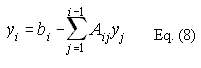
The summation of Eq. (8) represents the left hand side of node i. We are more interested on the right hand side (rhs) connections rather than the lhs. The next code uses rhs connections. Instead of solving for y[i] rightaway, we solve all y[s] incrementally. A code snippet shows how. This method is amenable to sparse matrix using lifo (last-in first-out) accessing because rhs nodes are also the nodes towards the bottom.
//forward course
Backward Course.
x[n]=x[n]/A[n][n]; <- The last node
3.4 Code Fragments on LUDM
Ax= b, let A= LU so
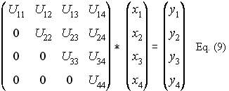
LUx= b, let Ux= y
Ly= b, solve y by forward course. Once y is know, solve for x in
Ux= y
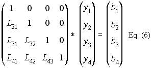
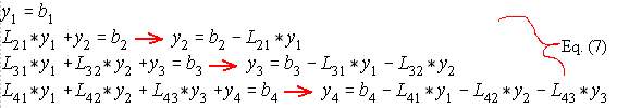
Vector y[] is just a temporary vector. We do not really have this stored in computer memory. We can solve for y[1] by multiplying row 1 of L-matrix with the column vector y[]. Do this also to row 2, row 3 and row 4. As you solve for y[2], y[1] is needed and that it is already solved. As you solve for y[3], you will need y[1] and y[2] and that they have been previously solved. See Eq. (7).
//Forward Course based on Eq. (8)
for (i=2; n; i++)
for (j= 1; j < = i; j++)
y[i]= y[i]- A[i][j]*y[j];
for (k=1; k < = n-1; k++)
for (i=k+1; i < = n; i++)
y[i]=y[i]-A[i][k]*x[k];
- - - - - - - - - - - - - - - - -
Let n=4, matrix size
k=1
i=k+1, n
y[2]=b[2]- L[2][1]*y[1]; <- y[2] is done here
y[3]=b[3]- L[3][1]*y[1]; <- y[3] and y[4] are not yet done
y[4]=b[4]- L[4][1]*y[1];
- - - - - - - - - - - - - - - - -
k=2
i=k+1, n
y[3]=b[3]- L[3][2]*y[2]; <- y[3] is done here
y[4]=b[4]- L[4][2]*y[2]; <- y[4] is not yet done
- - - - - - - - - - - - - - - - -
k=3
i=k+1, n
y[4]=b[4]- L[4][3]*y[3]; <- y[4] is done
By observation, only one y[] is finished for each loop of k, all other y[]s are slowly completed.
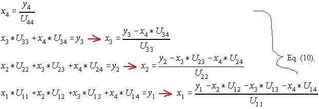
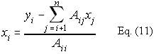
This code is an exact implementation of Eq. (11). This too is amenable to lifo accessing. Connections to node i represented by the summation are nodes belonging to the right hand side (rhs).
for (i=n-1;i>=1; i--)
{for (j=i+1;j < = n;j++)
x[i]=x[i]- A[i][j]*x[j]; //also as x[i]- =A[i][j]*x[j];
x[i]= x[i]/A[i][i]; //also as x[i]/=A[i][i];
}
Let us simulate the code.
x[4]=x[4]/A[4][4];
i=3
j=i+1,n
x[3]=x[3]-A[3][4]*x[4]; then x[3]=x[3]/A[3][3];
---------------------------------
i=2
j=3,n
x[2]=x[2]- A[2][3]*x[3];
x[2]=x[2]- A[2][4]*x[4]; then x[2]=x[2]/A[2][2];
---------------------------------
i=1
j=2,n
x[1]=x[1]- A[1][2]*x[2];
x[1]=x[1]- A[1][3]*x[3];
x[1]=x[1]- A[1][4]*x[4]; then x[1]=x[1]/A[1][1];
Let's mimic the forward course, i.e., incremental updating. This is not amenable to lifo because nodes going up are the same as lhs nodes.
for (i=n;i>=1; i--)
{x[i]= x[i]/A[i][i]; //division first, x[i] got already the summation
for (j=i-1;j>=1;j--)
x[j]=x[j]- A[j][i]*x[i];
}
And then simulate the code
i=4
x[4]=x[4]/A[4][4];
j=3,1
x[3]= x[3]- A[3][4]*x[4];
x[2]= x[2]- A[2][4]*x[4];
x[1]= x[1]- A[1][4]*x[4];
- - - - - - - - - - - - - - - - - - - - -
i=3
x[3]=x[3]/A[3][3];
j=2,1
x[2]= x[2]- A[2][3]*x[3];
x[1]= x[1]- A[1][3]*x[3];
- - - - - - - - - - - - - - - - - - - - -
i=2
x[2]= x[2]/A[2][2];
j=1,1
x[1]= x[1]- A[1][2]*x[2];
- - - - - - - - - - - - - - - - - - - - -
i=1
x[1]=x[1]/A[1][1];
None for j
In summary, the forward and backward course has to use a technique amenable to sparsity accessing.
