CHAPTER 2: Loadflow Solution by Gauss-Siedel Iterative.
GSLF_Fig 3
|
Applying the Nodal Equation in Power System
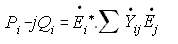
The current source in power systems comes from generated MW and MVAR. If our convention is an inductive Mvar for a lagging current, then apparent power in MVA=(complex conjugate V)* (I). By looking at the figure on the left, we assume that E has a positive angle and I has a negative angle with respect to the horizontal reference line. The angle of S is -(a+b). So S= P -jQ. It means that an inductive power has a negative Mvar. Note that E and V are synonymous notation for voltage.
|
What is an Iterative Process?
Suppose you want to get the square root of 100 just by division, a number being divided by another number. A simple code below shows how to perform an iterative process. An initial estimate next=1 is used. The correct answer is 10 and 1 is far from the answer. Then that initial estimate is used to divide the number. If the initial estimate is 10, the answer will be 10. But the answer is not correct, so we get the average of the initial estimate and the quotient. The difference between the initial estimate and the answer is called an error. This error must be less than the allowable error (tolerance) and we consider the answer as true to be correct. As the iteration continues, the error becomes smaller and smaller. This computation is called an iterative process. If the computation does not reach an answer it is said to be divergent, else it is convergent.
|
#include "stdio.h"   //replace the " with angle brackets
#include "math.h"    //incompatible with html coding
void main(void)
{double error=4, answer, next=1,number=100, toler=0.01;
 int iter=0;
 while (error>toler)
   {iter++;
    answer=(next + number/next)/2;
    error=fabs(next-answer);
    printf("iteration:%2d  next=%7.3f ",iter,next);
    next=answer;
    printf("answer=%7.3f  error=%7.3f\n",answer,error);
    }
}
iteration: 1  next=  1.000 answer= 50.500  error= 49.500
iteration: 2  next= 50.500 answer= 26.240  error= 24.260
iteration: 3  next= 26.240 answer= 15.026  error= 11.215
iteration: 4  next= 15.026 answer= 10.840  error=  4.185
iteration: 5  next= 10.840 answer= 10.033  error=  0.808
iteration: 6  next= 10.033 answer= 10.000  error=  0.033
iteration: 7  next= 10.000 answer= 10.000  error=  0.000
|
Gauss-Siedel Loadflow (GSLF)
 |
GSLF_Eq. 4 on the left is the representation of GSLF_Eq. 3. Substituting Eq. 4 in Eq. 5 yields Eq. 6. This equation can be visualized using a sample 4-bus system as shown on Fig. (4).
|
| Ybus for power system is in complex number.
to get the real part, multiply and divide with its conjugate. This will make the denominator in real numbers only.
GSLF_Fig 4
|
| By definition, the off diagonal has negative of the line admittance and the diagonal is the sum of admittance connected to the node.
With this procedure, we do not use sin() and cos(). Since bus-4 has no connection to bus-1, so there is no entry for Y(1,4). This is also true with Y(4,1). For a power system with something like 1000 nodes, each node can have an average of 4 connections thus the Ybus can have a 95% zero values. Note that the diagonal is always nonzero.
|
| This set of simultaneous equations is considered non-linear, compared with GSLF_Eq. (3) of the previous chapter. The state variables are the voltages and these are the unknown. When the E on the denominator of the lefthand side is transferred to the right hand side, you have a product-- which makes the equation non-linear.
GSLF_Fig 7
|
We can write a general equation for nodes 1 to 4 from Eq. (7),
 GSLF_Fig 8
The summation above includes when i=j. Mark this equation as all power system algorithms are based on it. This equation is called "injected power on bus i".
A method called Gauss-Siedel can solve the unknown voltage, first by assuming a guess say E=1.0 for all. Then that value is improved by substituting them to the rest of the equation. By examining node 3, in Eq. (7),for example, E(3) is on the left side as the denominator of (P -jQ) and as the diagonal of the right side.
|
To apply the Gauss-Siedel iteration, we equate the YiiEi (diagonal) as the unknown voltage. Let us transpose and solving for E(3), and generalize with subscripts i,j,k as shown in GSLF_Eq. 9. Here, i is the node we are solving and j's represents the nodes connecting node-i and k represents the iteration counter. The left side of node-i are the voltages we already updated and the right side of the diagonal have voltages whose value are computed
GSLF_Eq. 9.
|
from the previous iteration represented by superscript (k-1). The voltage at the denominator of (P -jQ), which is also for node-i has its value based on (k-1). Since we do not store the old voltage from the updated voltage, the programming aspect will just be simple. If we use rectangular coordinates for Yij as (g +jb) and E as (e +jf)
|
we can avoid the use of trigonometric sin(), cos() and atan() functions.
GSLF_Eq. 10 represents the dissected portion for (RePQE +j ImPQE). Pi here is the injected power which is the generated MW minus the demand MW. Since the denominator is a conjugate of Ei, it is equated to (e -jf). To remove the j part from the denominator, it must be multiplied and divided by its conjugate which is (e +jf).
GSLF_Eq. 10.
|
| This portion is the summation Yij*Ej. It does not include the diagonal part. In the for loop, it exclude j=i.
GSLF_Eq. 11.
|
Re= RePQE - ReSumYE
GSLF_Eq. 11.
Im= ImPQE - ImSumYE
Performing the last part
 GSLF_Eq. 13.
Program Listing_1: Gauss-Siedel Loadflow
This is a beginner's code because the Ybus matrix is full or in 2 dimension. Node numbering is contiguous starting from 1.
Code Explanation:
|
The code has 4 main subroutines
input();---read line and bus data. Also forms the Ybus matrix which
       includes line charging in MVAR. How is Mvar line charging
       converted to admittance?
       S=E*I, I=E/Z, S=E.E/Z, Z=E.E/S, Y=S/E.E
       Because of pi representation and E=1.0 pu when that charging was
       computed, so Y=S/(base*2) pu (mho).
gsiedel();---iterate voltage. The error being watched here is the change
        in voltage both in real and imaginary part. That maximum error is
        checked against a tolerance usually 0.0001. To prevent divergence,
        iteration count should not exceed some value. Check for PV-type bus
        will be discussed later.
pflows();---solve power flows. This is performed after the iteration is
        completed. Discussion of the equation follows.
gener();---solve generation, Pg,Qg=SL, Qg=PV.
|
Line Flows
As discussed above, the system of equations can be solved with any combination of Y and E as shown below. Those with polar Y and/or E will use trigonometric functions.
polar Y
polar E | polar Y
rectangular E | rectangular Y
polar E
| rectangular Y
rectangular E
|
GSLF_Fig 5.
|
Using rectangular Y and polar E, line flow equations will be derived. Based from Fig. (5), there are 2 components of current from node 1: due to the line impedance and due to line charging. Assuming node 1 is of a higher potential than node 2, current is from 1 to 2. There are things to remember on Eq. (13). The line admittance is not stored separately. It is taken from Ybus. But Yij is defined as negative of line admittance, so take it from Ybus and negate it.
|
Line impedance is inductive and is defined as (r +jx), so a line capacitance is (-jx). The reciprocal of line charging is therefor (+j). And of course the complex conjugate of E has its voltage angle negated. GSLF_Eq. 14 shows in general notation for a flow from node-i to node-j.
 GSLF_Eq. 13.
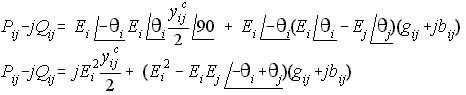 GSLF_Eq. 14,15.
Eq. (15) is the result after collecting angles from Eq. (14)
Performing the multiplication of the last quantities and with a review of trigonometric functions as shown on Eq. (17),
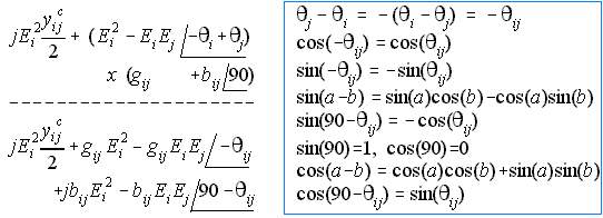
GSLF_Eq. 16(left), 17(right).
We now expand the complex terms into a real and imaginary part.
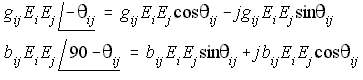 GSLF_Eq. 18.
Collecting the real terms and equate them to Pij and the imaginary terms to Qij results to Eq. (19). The shunt on Qij may be replaced with shunts from off-nominal transformer tap.
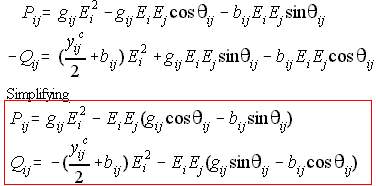 GSLF_Eq. 19.
Solving for Generated MW, MVAR
| Once the iterative process has converged, it is now ready to solve for Pg,Qg of the Slack bus, and Qg for PV-type bus using a derived formula based on Eq. (5). Total MW and MVAR loss is also computed by the same equation. Then solve for system mismatch. Mismatch is an error in MW/MVAR affected by the chosen convergence tolerance. Mismatch=(Total Generation)- (Total loss + Total load).
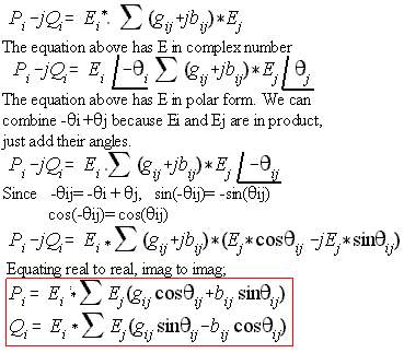
Eq. (5) is in matrix form. We will derive the injected real and reactive power using polar E and rectangular Y. This derived Eq. (20) will be used in Newton-Raphson, Fast Decoupled and Optimal Loadflow. The gif on the left shows how.
GSLF_Eq. 20.
|
| Alternate derivation using rectangular E and Y. We need this in solving for Qg of PV type bus inside the Gauss-Siedel iteration.
GSLF_Eq. 21.
|
Program Listing_2: Gauss-Siedel Loadflow with LIFO
Code Explanation: This code is a bit advance because the off-diagonal elements of the Ybus matrix is stored like line data whereas, the line impedance is not stored. The diagonal part is stored in parallel with the bus data. To perform the summation in Eq. (10), lifo is used. Details on this data structure can be found in "Part 1: Short Circuit, Chapter 6".
