| |
CHAPTER 4: Newton-Raphson Loadflow (NRLF)
Unlike Gauss-Siedel, (GS) which updates the node voltage one at a time, Newton Raphson, (NR) solves a voltage correction for all the nodes and update them. A simultaneous linear equation in the form of Ax=b is evaluated each iteration. Look again on "Program Listing_1: DC Circuit Flow" on how to solve Ax=b by Gauss-Jordan Reduction.
Comparing NR with GS, GS has problems when the system becomes large. One reason is the presence of negative impedance as a result of transformer 3-winding representation. GS tends to increase in iteration count and is slow in computer time.
Let us solve a sample 2 equations in 2 unknowns and non-linear.
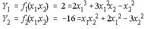 NRLF_Eq. (1) NRLF_Eq. (1)
Set an initial estimate, get a correction, update the estimate. By Taylor Series Expansion;
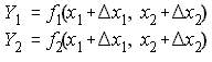 NRLF_Eq. (2) NRLF_Eq. (2)
can be expanded to
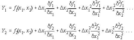 NRLF_Eq. (3) NRLF_Eq. (3)
Eq. (3) can be expanded to 3,4,etc as the exponent. The last 2 terms of the 2 equations have x in exponent 2 and the derivatives are in second order. By neglecting these last 2 terms, we get only the linear partial derivatives. This is just an ordinary derivative.
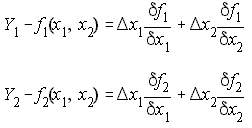 NRLF_Eq. (4) NRLF_Eq. (4)
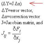 | Eq. (4) can be written in matrix form as shown on the left with the red arrow. This is in the form of Ax=b. Instead of solving the simultaneous non-linear equations, we are now solving simultaneous linear equations.
NRLF_Eq. (5)
|
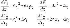
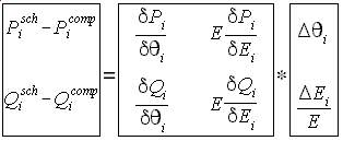
| Performing the derivatives on Eq. (1), yields the elements of the Jacobian matrix. The error vector is the difference between the scheduled value and the computed value when the state variables are substituted to the set of equations. The unknown is the correction to the state variables.
| 
NRLF_Eq. (6)
|
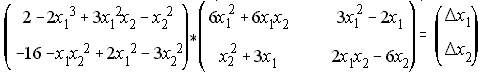 |
Eq. (7) is the matrix representation of Eq. (4).
NRLF_Eq. (7)
|
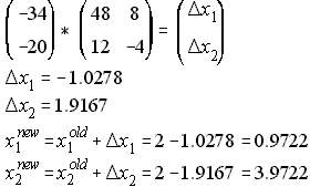
Iteration=1:
Let x(1)=2,x(2)=2 be the initial estimate. Substituting to Eq. (7), and solving for the correction and updating x(1),x(2) yields;
 NRLF_Eq. (8) NRLF_Eq. (8)
Iteration=2:
Substitute again the updated x(1),x(2) to Eq. (7), and solving for the correction and updating x(1),x(2) yields;
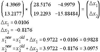 NRLF_Eq. (9) NRLF_Eq. (9)
This is to be continued until the error vector is less than some tolerance.
Derivation of NRLF Formula
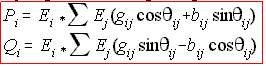 | This equation was taken from GSLF_Eq. (20). From the above 2 equation sample, this is similar to Eq. (1). NRLF_Eq. (10) bus injected power
|
Comparing to Eq. (1), the numbers 2 and -16 are the actual values when x(1) and x(2) are substituted on the equations. Similarly, when the computed voltages are applied to Eq. (10), it should result to the scheduled value of generated power less load. But because there is some degree of error, then there is some mismatch. The error vector then becomes the scheduled injected power less than the computed injected power. The state variables are the voltage and the voltage angle, so the correction vector will be delta theta and delta e. If there are 2 nodes, there will be 4 state variables. So the size of the Jacobian matrix is 4x4.
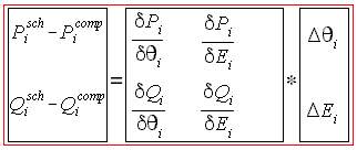 NRLF_Eq. (11) NRLF_Eq. (11)
Eq. (11) can be re-written as Eq. (12)
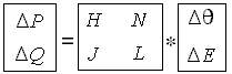 NRLF_Eq. (12) NRLF_Eq. (12)
We now derive the elements of each submatrices H,J,N and L.
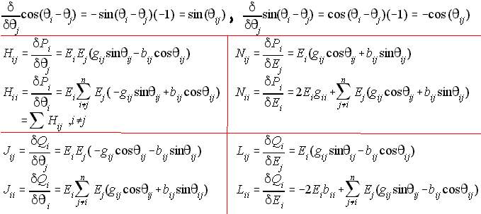
NRLF_Eq. (13)
Eq. (10) includes when j=i. It means that the diagonal of the Ybus is included. When taking the derivative of variable-i with respect to variable-j, there is only one node-j in the summation symbol. So the resulting derivative has no summation symbol. Whereas taking the derivative of i with respect to i, the summation symbol is included. There exists a product term of i to j. At the bottom of the summation, it says j is not equal to i. Taking a derivative with respect to theta when j=i simply is non existant because theta is zero. However, when taking the derivative with respect to E, there is a value even if theta is zero because cosine of zero is 1, while its sine is zero.
Some Improvement to NRLF
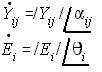
By multiplying N and L with E and dividing delta E with E, computing time can be reduced. The code is simplified too.
 NRLF_Eq. (14) NRLF_Eq. (14)
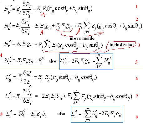 | The red numbers from 1 to 9 are for explanation purposes only. In line 2 the one term of 2EiEiGii is transferred inside the summation to satisfy when j=i. The summation portion now becomes the computed injected real power. Also the summation portion is equal to N'ij as shown in line 5. This is also true to line 7. One part of -2EiEiBii is thrown inside the summation which is equal to the computed reactive power injection.
NRLF_Eq. (15)
|
SUMMARY OF FORMULA FOR H,J,N',L'   The prime in N and L is not
Hij=EiEj(GijsinOij - BijcosOij)              shown in the code.
Hii=-sumHij, j.ne.i                        note: O is for theta

Nij=EiEj(GijcosOij + BijsinOij)
Nii=2EiEiGii + sum Nij,  j.ne.i

Jij=-Nij
Jii=Nii - 2EiEiGii

Lij=Hij
Lii=-Hii - 2EiEiBii
deltaPi=Pi(sch)-Nii +EiEiGii       delta is for error
deltaQi=Qi(sch)+Hii +EiEiBii       sch=generated-load

COMPUTER IMPLEMENTATION
loop i
   loop j
       1. Hij=EiEj(GijsinOij - BijcosOij)
       2. Nij=EiEj(GijcosOij + BijsinOij)
       3. Jij=-Nij
       4. Lij=Hij
       5. Hii-=Hij     this is a C/C++ code
       6. Nii+=Nij
   next j
   7. Jii=Nii   //Nii is not complete yet
   8. Nii+=2EiEiGii
   9. Lii= -Hii -2EiEiBii
  10. deltaPi=Pi(sch)-Nii +EiEiGii
  11. deltaQi=Qi(sch)+Hii +EiEiBii
 next i

IMPROVED PSEUDO CODE
This will require a single sweep on line data and a single
loop on bus data. Gij,Bij can be stored along np[],nq[]

loop k=1,lines
    i=np[k]; j=nq[k];
    EiEj=E[i]*E[j];
    Oij=O[i]-O[j];
    Oji=-Oij;
    Hij=EiEj*(Gij*sin(Oij)-Bij*cos(Oij));  Not symmetrical
    Hji=EiEj*(Gij*sin(Oji)-Bij*cos(Oji));
    Hii-=Hij;
    Hjj-=Hji;
    Nij=EiEj*(Gij*cos(Oij)+Bij*sin(Oij));
    Nji=EiEj*(Gij*cos(Oji)+Bij*sin(Oji));
    Nii+=Nij;
    Njj+=Nji;
    Jij=-Nij;
    Jji=-Nji;
    Lij=Hij;
    Lji=Hji;
next k
loop i=1,nbus
    EiEi=E[i]*E[i];
    Jii=Nii;  //Nii is not complete yet
    Nii+=2EiEi*Gii;
    Lii=-Hii-2EiEi*Bii;
    deltaP[i]=Pi(sch) -Nii +EiEi*Gii;
    deltaQ[i]=Qi(sch) +Hii +EiEi*Bii;
next i
Program Listing_1: NEWTON RAPHSON LOADFLOW
- with row/col delete to solve Ax=b
|
Code Explanation:
There is no need to store the Ybus matrix as a square. The formation of HJNL uses a single sweep on the line data and the Ybus elements are accessed in that order. The diagonal is stored with the bus data. The Jacobian matrix is coded with bus type in vector tcol[2*nb] and bus number in vector tnum[2*nb]. Remember that the matrix size is twice the bus data. Column and row entries for Slack and PV bus are deleted to simulate how to do it using a calculator. The bus number code tnum[] is also deleted for the entry of Slack and PV type. Update of voltage angle and magnitude are only for those nodes in tnum[].
Program Listing_2: NEWTON RAPHSON LOADFLOW
- no delete to solve Ax=b
Code Explanation: The solution of Ax=b does not actually delete row/column due to slack bus. In order to visualize the process of factorization, we have included Listing-1. Shown below will be the modification in Listing-1 and -2 if we have to include PV busses. In Listing-2, just ignore the row and column after nb (nb=number of nodes) for PV busses. PV bus does not get a voltage update.
Newton Raphson Using the Algorithm by Van Ness
The Jacobian matrix is in rectangular and updating voltage and angle is in polar. Let
 NRLF_Eq. (16) NRLF_Eq. (16)
The equation above shows the polar form of the Ybus. This is needed in the derivation of formula which is tricky.
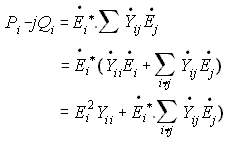 NRLF_Eq. (17) NRLF_Eq. (17)
Rewriting GSLF_Eq (5) and taking out the term when i=j is shown above. The summation simply means that we are substituting the non-zero elements of row=i from the Ybus. The first summation does not contain (i not equal to j), so it includes the diagonal of the Ybus. The next 2 summations excludes when i=j. The dot above the variable refers that it is a complex number. The asterisk means that we take the conjugate of the complex number. We can now separate the real part and equate it to the real part of the right hand side term. Yii is composed of Gii and jBii.
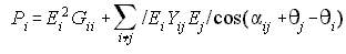 NRLF_Eq. (18) NRLF_Eq. (18)
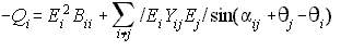
Transferring the negative sign,
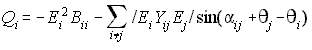 NRLF_Eq. (19) NRLF_Eq. (19)
From Eqs (18) and (19) we can simplify the derivation process, let A and B be substituted to as shown below,
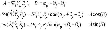 NRLF_Eq. (20) NRLF_Eq. (20)
The purpose of the above Eqs (18) and (19) is to equate Pi and Qi in terms of  and be able to get the derivatives of Pi and Qi with respect to and conform with the definition of the Jacobian matrix. The tricky part is that we will not use the sine and cosine terms. Watch on. and be able to get the derivatives of Pi and Qi with respect to and conform with the definition of the Jacobian matrix. The tricky part is that we will not use the sine and cosine terms. Watch on.
Now let us get the rectangular parts of 
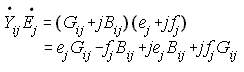 NRLF_Eq. (21) NRLF_Eq. (21)
 NRLF_Eq. (22) NRLF_Eq. (22)
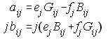
For simplification, aij, bij is substituted,
 NRLF_Eq. (23) NRLF_Eq. (23)
We can now equate real part to real part, and imaginary part to imaginary part.
 NRLF_Eq. (24) NRLF_Eq. (24)
 NRLF_Eq. (25) NRLF_Eq. (25)
Eqs (18) and (19) can now be replaced with these new derived values. We will need Eq (26) in the programming code.
 NRLF_Eq. (26) NRLF_Eq. (26)
The method of Van Ness is different from the ordinary Newton Raphson, because he group individual H,N,J,L for branch i-j near each other instead of 4 separate sub-matrices.
 NRLF_Eq. (27) NRLF_Eq. (27)
 NRLF_Eq. (31) NRLF_Eq. (31)
We now get the derivatives. I hope you know how to. The aspect of this website is to show the reader how to create the industry grade programming aspect, rather than the details of the mathematics involved.
 NRLF_Eq. (32) NRLF_Eq. (32)
 NRLF_Eq. (33) NRLF_Eq. (33)
 NRLF_Eq. (34) NRLF_Eq. (34)
 NRLF_Eq. (35) NRLF_Eq. (35)
Eqs (24) and (25) will be used instead of the sine and cosine terms to form the H,N,J,L.
We are now ready to show the programming code.
COMPUTER IMPLEMENTATION
loop k=1, Lines
   i=pbus[k]; j=qbus[k];
      1. aij=e[j]Gij - f[j]Bij;  aji=e[i]Gij - f[i]Bij;
      2. bij=e[j]Bij + f[j]Gij;  bji=e[i]Bij + f[i]Gij;
      3. ReEYEij=e[i]aij + f[i]bij;  ReEYEji=e[j]aji + f[j]bji;
      4. ImEYEij=e[i]bij - f[i]aij;  ImEYEji=e[j]bji - f[j]aji;
      5. Hij= -ImEYEij; Hji= -ImEYEji;
      6. Nij=  ReEYEij; Nji=  ReEYEji;
      7. Jij= -ReEYEij; Jji= -ReEYEji;
      8. Lij= -ImEYEij; Hji= -ImEYEji;
   collect Pi, Qi
      9. Pi = Pi + ReEYEij;   Pj = Pj + ReEYEji;
      10.Qi = Qi + ImEYEij;   Qj = Qj + ImEYEji;
 next k

 loop i=1, Nodes
   11. Hii=Qi   //Qi is not complete yet
   12. Jii=Pi   //Pi is not complete yet
E[i] squared = e[i] squared + f[i] squared
Let E2=e[i]e[i]+ f[i]f[i]
   13. Pi=  Pi + (E2)Gii
   14. Qi= -Qi - (E2)Bii
   15. Nii= Pi + (E2)Gii
   16. Lii= Qi - (E2)Bii
 deltaP[i]=Pi(sch) -Pi;
 deltaQ[i]=Qi(sch) -Qi;
next i
|
Program Listing_3: NRLF by Van Ness Algorithm
- no delete to solve Ax=b
Code Explanation: This code simulates the algorithm used by a full blown Newton Raphson made by PECo. We can learn plenty of things by analyzing how a successful program implements area control, tap-changing under load transformer, PV busses hitting its limits and others.
|
