3.1 Shipley-Coleman Matrix Inversion.
This inversion does not augment a matrix by a unity as in Gauss-Jordan.
Inversion is being done utilizing the matrix itself. It is an "in-place" inversion, just
like the "Gauss-Jordan In-place Inversion". Unlike the latter, the formula derivation
is simple. We will use this inversion routine in full matrix even for production
grade software because matrix size is just 20x20. This routine is used to invert the
primitive coupling impedance matrix [z]. See Ref. 9.
3.2 Mathematical derivation.
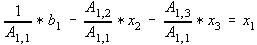
Loop 1: From Eq. 1 transfer x1 to RHS (right hand side)
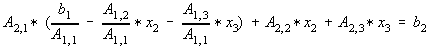
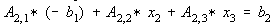
Loop 2: From Eq. 8, solve for x2,
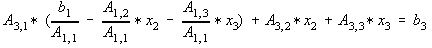
Doing the same for Loop 3 will result into the form,
where from 3.3 Procedure for Computer Implementation.
3.4 Computer Program (SHIPLEY.C), Input/Output
3.1 Shipley-Coleman Matrix Inversion
3.2 Mathematical Derivation
3.3 Procedure for Computer Implementation
3.4 Computer Program (SHIPLEY.C)
3.5 Example Calculation Output
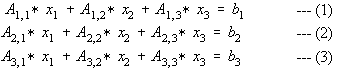
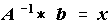
From A*x=b, we would like to manipulate A to arrive on
 ,
,
where A is a n x n matrix, and b and x are vectors of n size.
Consider a size 3 x 3.
 --- (4)
substitute Eq. 4 to Eq. 2, i.e.,
collecting terms,
 --- (5)
Also substitute Eq. 4 to Eq. 3,
collecting terms,
 --- (6)
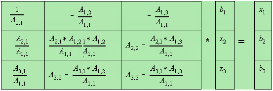
Rewriting Eqs. 4,5,6 in matrix form;
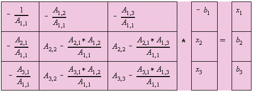
Multiply column 1 by -1 and  by -1 does not alter the matrix.
The reason for such will be made clear during the programming aspect.
by -1 does not alter the matrix.
The reason for such will be made clear during the programming aspect.
After the necessary calculations, each element in the A matrix would change as
indicated by the matrix above. It can be again rewritten as;
where the elements Ai,j are now different from Eqs. 1,2,3.
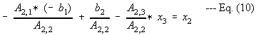
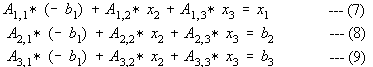
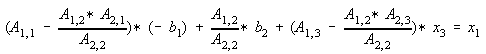
Substitute Eq. 10 to Eq. 7,

Collecting terms,
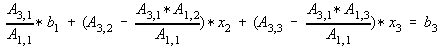
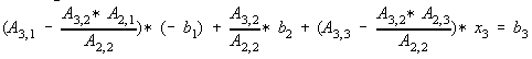
Substitute Eq. 10 to Eq. 9,

Collecting terms,
Writing in matrix form and multiplying column 2 by -1 and b2 by -1,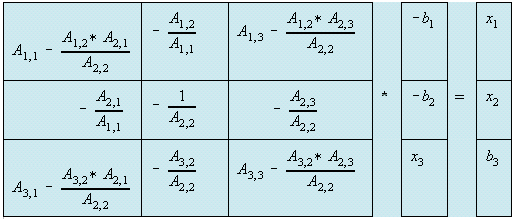 --- Eq. (11)
 --- Eq. (12)
 ,
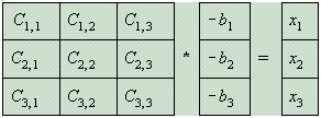
Eq. 12 can be transformed as [-C]*[b] =[x]
by multiplying [b] by -1 and[C] by -1, so
,
Eq. 12 can be transformed as [-C]*[b] =[x]
by multiplying [b] by -1 and[C] by -1, so
 .
.
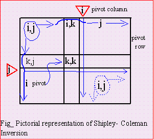
Generally, with Shipley inversion you can search the largest diagonal to act as a
pivot, similar to Gauss-Jordan in-place inversion. However, in short circuit
applications, there is no need for such diagonal search. In power system analysis, diagonal elements of any matrix is said to be dominant. Its value is greater than the off diagonal elements. The code to implement the
method is given below. Note on the minus sign as previously done in the derivation.
 /**********************/
 /*Shipley_Inversion();*/     CODE SNIPPET
 /**********************/
 1:  for (k=1;k<=z_size;k++)
 2: // the pivot element
 3:   { A[k][k]= -1/A[k][k];
 4:
 5: //the pivot column
 6:    for (i=1;i<=z_size;i++)
 7:        if (i!=k) A[i][k]*=A[k][k];
 8:
 9: //elements not in a pivot row or column
 10:     for (i=1;i<=z_size;i++)
 11:        if (i!=k)
 12:            for (j=1;j<=z_size;j++)
 13:                      if (j!=k)
 14:                          A[i][j]+=A[i][k]*A[k][j];
 15:
 16: //elements in a pivot row
 17:    for (i=1;i<=z_size;i++)
 18:       if (i!=k)
 19:            A[k][i]*=A[k][k];
 20:   }
 21:
 22: //change sign
 23:   for (i=1;i<=z_size;i++)        /*reverse sign*/
 24:     for (j=1;j<=z_size;j++)
 25:        A[i][j]=-A[i][j];
We can understand the code segment by comparing Eq. (11) with the pictorial
representation and the code. The inversion has the outermost k-loop. To minimize
the amount of arithmetic operations, the pivot has its negative reciprocal stored at
line_3. Then computed next is the pivot column except of course the pivot A[k][k],
that is the test on line_7. The pivot row is not computed next, because its value
without the denominator A[k][k] is needed. Otherwise, we would have the
denominator twice for the elements not in the pivot-rows and columns. In line_14
pivot-col A[i][k] had been an updated value and pivot-row A[k][j]) is not. While
Eq. (11) says it is a divide for pivot row, Line_19 is a multiplication and also with
Lines_14 and _7 because we have done the division already in Line_3.
HOME
CHAPTER ONE: INTRODUCTION
CHAPTER TWO: PROGRAMMING TOPICS
CHAPTER THREE: MATRIX INVERSION ROUTINE
CHAPTER FOUR: STEP-BY-STEP ALGORITHMS
CHAPTER FIVE: DIRECT METHODS IN Ybus FORMATION
CHAPTER SIX: SPARSITY
CHAPTER SEVEN: MATRIX FACTORIZATION AND OPTIMAL ORDERING
CHAPTER EIGHT: SPARSE Zbus FROM FACTORED SPARSE Ybus
CHAPTER NINE: FAULT CALCULATIONS
REFERENCES
