6.1 Sparsity Techniques.
6.1 Sparsity Techniques
6.2 Single-Entry Table
6.3 Double-Entry Table
6.4 Last-in First-out Linked Lists (LIFO)
6.5 Formation of the Linked Lists
6.6 Computer Program (LIFO.C)

This topic is needed in understanding how fill-ins are minimized during LU Factorization. Large scale power systems have a small number of transmission lines connected to each substation. Only few elements of the Ybus are non-zero, corresponding to lines or transformer connections. Such matrix is said to be sparse. From the viewpoint of programming, i.e. computer speed, accuracy and data storage it is desirable to perform calculations only on the non-zero entries of the Ybus. In the process of solving Ax=b, there is a need of accessing all nodes connected to a particular node in question. Or simply, what are the non-zero elements in a particular row? This can be done using 3 methods shown below. There may be other methods in the literature. These sparsity techniques of data accessing is also used in other power system application programs.

1. Single-Entry Table, so simple
2. Double-Entry Table
3. Last-in First-out Linked Lists (LIFO)

6.2 Single-Entry Table.

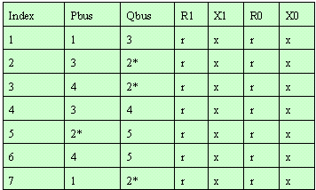
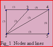
The branch data for short circuit calculation consists of the positive sequence resistance and reactance (R1,X1), as well as its zero sequence (R0,X0). The branch data for Fig_1 will be;

Table 6.1

We would like to know all nodes connected to 2. By looking at the figure, these nodes are 3,4,5, and 1. In order to get these elements, the program has to search the arrays pbus[ ] and qbus[ ] for a node 2, those with asterisk(*) in the table. The opposite nodes become its first neighbors. This single-entry table is time consuming since there is a need to test the entire branch list for every node-i processed.

6.3 Double-Entry Table.

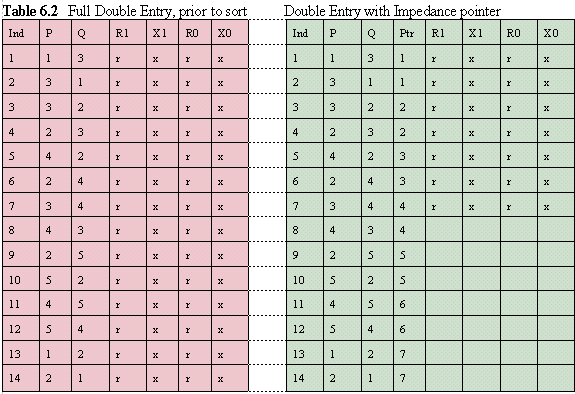
The single-entry table is duplicated and sorted. All arrays now will be twice as large. A location pointer can reduce memory storage by not duplicating the entry of the sequence impedances (R1,X1,R0,X0).

After sorting the branches with pbus[ ] as its key, the table will now be;

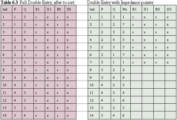
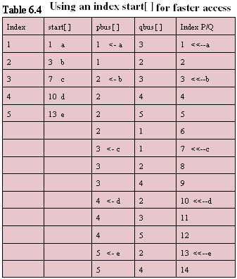
The impedance table of the Full-Double-Entry is also sorted, i.e., with data movement. The Double-Entry with pointer has its impedance table no data movement and only half storage as the former. The qbus[ ] side may also be sorted if the qbus[ ] side are the same. The sorted form is necessary in the output of branch contributions. From the table, the nodes connected to 2 are 3,4,5, and 1. For large systems, it will be time consuming to find the start and end of branches connected to node-i. To avoid searching for the start and end of thread, another vector is needed to store the start of thread. Its value is searched from the index for the first location of the said node. Its ending is not stored anymore as it can be computed by subtracting 1 from the next node. Care must be considered for the last node as there is no next node for it. In this example, the value for such vector is;

Time consumption is reduced in accessing all nodes connected to node-i. The code for this will be; for (i=start[i]; i<=start[i+1]-1;i++)     {n=qbus[i] // all n's are the desired nodes     etc...     } With the vector start[ ], we can now delete vector pbus[ ], as it is no longer needed. However, we must add index=6 as, start[6]=15. This double-entry is an improvement from the single-entry table, however the LU Factorization of Ybus (or B' and B'' of Loadflow), an insertion of pbus[ ]/qbus[ ] is needed for a fill-in. A fill-in is now a non-zero value when previous to the factorization, it was zero (more on this on the next chapter). In short circuit, it can also be a result when a coupling matrix for a group is applied to the zero sequence Ybus. Data movement itself is needed to retain the sorted form of pbus[ ] and also start[ ] has to be modified for nodes I+1 to NBUS.

Data movement is time consuming. Method 4 will solve this problem. A programming technique is used by PECo to reduce computer storage and execution time. pbus[ ] and qbus[ ] is stored using 2 bytes only. Maximum integer size is 65535 (2 exp 16-1). Both pbus[ ] and qbus[ ] is stored in a single 4 bytes integer. It is something like,

INTEGER*4 LINEF(2500), NPQ INTEGER*2 NP(2), PBUS, QBUS EQUIVALENCE (NPQ,NP(1)) . . READ( ) PBUS,QBUS etc NP(1) = PBUS NP(2) = QBUS icount= icount + 1 LINEF(icount) = NPQ c----- NP(1) = QBUS NP(2) = PBUS icount= icount + 1 LINEF(icount) = NPQ

Sorting will be done only on array LINEF( ).

6.4 Last-in First-out Linked Lists (LIFO). The entry of pbus[ ] and qbus[ ] is arbitrary. A sorted form of pbus/qbus can be realized without data movement on the branch impedances. Fill-ins can be inserted without data movement too. The following arrays are needed; start[i] = pointer to the beginning of the list of nodes connected to i. The size of this vector is NBUS, the number of nodes. next[ ] = pointer to the next entry in the branch table. The size of this vector is 2 x LINES, where LINES is the number of branches. mbus[ ] = list of nodes connected to i. Size is also 2 x LINES. This corresponds to the original pbus[ ]/qbus[ ]. R1[ ],X1[ ],R0[ ],X0[ ] =are the same branch impedance. Size is LINES.

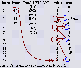
Only start[ ] and next[ ] are added to the single-entry table, totalling to NBUS + 2*LINES integer words. Note that mbus[2*LINES] corresponds to the sum of the sizes of pbus[LINES] and qbus[LINES]. This is an advantage over the double-entry table on the memory requirement. The vectors start[ ], next[ ] and mbus[ ] are built as the data are read in to form a last-in first-out or stacks for each node. When completed, they allow to find all the branches connected to node i. Each start[i] entry points to one end of the thread (top of the stack) for the corresponding node-i. The corresponding next[ ] element points to the next (previously entered) connection to this same node. A zero in next[ ] indicates the end of the thread. Data is found at half the position of the mbus[ ] entry, rounded up to the next integer, if necessary. The best advantage of Lifo is that there is no data movement during an insertion of a fill-in.

The linked list for the same network is shown below when data is completed.

As an illustration, suppose we would like to get the nodes connected to 2, please see Fig_2..

start[2]= 14 location of node 2 says starting node is at index 14. mbus[14]= 1 It says node 1 is connected to 2. next[14]= 9 NEXT is pointing to index 9. mbus[9]= 5 Node 5 is another node connected to 2. next[9]= 6 pointing to index 6 again. mbus[6]= 4 Node 4 is another node. next[6]= 4 pointing to index 4 again. mbus[4]= 3 Node 3 is another node. next[4]= 0 ** end of thread **.

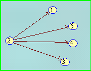Fig_2.

6.5 Formation of the Linked Lists.

The start[ ], next[ ] and mbus[ ] vectors are formed be examining the entries in pbus/qbus, branch by branch, adding 2 entries to next[ ] and mbus[ ] for each branch, and changing the appropriated start[ ] elements to point to the latest additions. The elements added to next[ ] are made to point to positions previously added to the threads, if any. That is, they are made to point to the positions which the start[ ]s pointed to before the latest branch was added. The table below shows when branch 1-4 had been read in and branch 5 is about to be added.

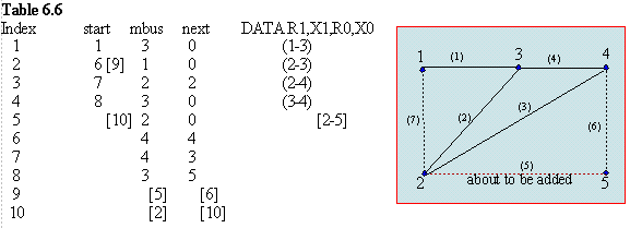
Note that the vectors next[ ], mbus[ ] and DATA are the same as in Table 6.5, while in start[ ] are different. Now examine branch 5 on Fig. 6.2. The next open position in Table 6.6 is index 9. Taking pbus[5]=2 first, the other end bus number is qbus[5]=5, so mbus[9] is set to 5. This branch is part of the thread for node=2 and it must now be linked-in. To do this, the pointer from start[ ] to next[ ] is moved to next[9],

next[9] = start[2] = 6
and start[ ] is pointed to the new line, start[2] = 9.
Similarly, from the viewpoint of bus 5 in index 10,
mbus[10] = pbus[5] = 2
next[10] = start[5] = 0
start[5] = 10

The changes are shown in [ ] as branch (2-5) is added. start[ ] elements always point to the last element added to a row, thus producing a last-in first-out list or stack (LIFO). Each next[ ] element points to a previous entry or else zero, indicating the end of a thread. The location of data must be found as one searches a thread. This is done by an integer division,
J = (LK + 1)/2

where LK is the index of the other end bus entry in mbus[ ]. Say, for example, that the branch had originally been entered in positions 5 and 6 of the linked lists. The data went in position 3. The integer division will find the same data position no matter which of the linked list positions belong to the particular thread,i.e.,
J = (5 + 1)/2 = 6/2 =3
J = (6 + 1)/2 = 7/2 =3.

6.6 Computer Program. (LIFO.C)

Some Code Comments

Without line numbers comments and printing, the lifo formation would simply look:
read(p,q,ckt,x1,x0);
next[++count]=start[p]; start[p]=count; mbus[count]=q;
next[++count]=start[q]; start[q]=count; mbus[count]=p;

To access connectivity to node-i, i.e. all nodes connected to i, the code would be:
more=start[i];
while (more)
   {p=mbus[more];
   more=next[more];
   }
Lifo formation and retrieval is incredibly simple and yet powerful because as mentioned earlier, you can sort branch flows and insert fill-ins without ever moving the impedance Ybus or Zbus data.

Program Input/Output
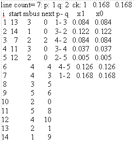
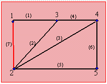
Shown below is the input data with 7 branches. As each branch is read a lifo is formed and printed with corresponding graph. All dotted lines are not yet read.

1 3 1 .084 .084
3 2 1 .122 .122
4 2 1 .084 .084
3 4 1 .037 .037
2 5 1 .005 .005
4 5 1 .126 .126
1 2 1 .168 .168
99 0 0 0 0

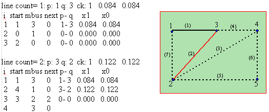
The drawing on the right corresponds when the second branch is read.

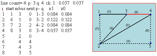
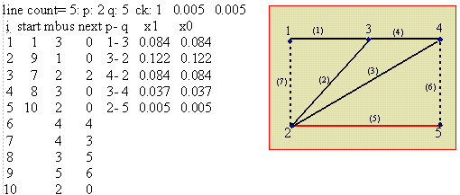
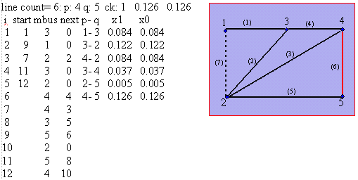
DOWNLOAD C# lifo.zip file just click choose Save