The building of algorithm of the zero sequence Zbus is complicated by the existence of mutual coupling. As each line is selected from the reordered line list for processing, it is checked against
the list of coupled lines. If
it is uncoupled, the line is processed using Types 1,2,3,4. If the line is found in the coupling list, a further check
is made if it is the first line of the coupled group. Types 1,2,3,4 is used if it is the first line in the group.
However, if the line to be added is coupled to line/s in the partial network, the modification of Zbus must take
into account the mutual coupling.
4.13 Type 5 Modified Branch Algorithm.
| 
| --- Eq. (1)
|
A line has been selected from the data list and has
been found to be mutually coupled to line/s in the partial
network PN. The line to be added is line PQ, where P is in PN. See Fig_1.
Line PQ is mutually coupled to one or more lines RS (here RS is
the running index). The relationship that applies to new line
PQ and the several lines to which it is coupled is given by I=Y*V
(coupling equation) is;
Injection of 1.0 pu current into bus k will produce
 since line PQ is not part of the mesh. So,
 --- Eq. (2)
 --- Eq. (3)
Since the voltage across a line is equal to the difference of voltage of the busses at the ends of the line,
Substituting Eq.(4) to Eq.(3),
 --- Eq. (6)
where from Eq.5,
 ---Eq. (7)
Substituting Eq. (7) to Eq. (6),
 ---Eq. (8)
Rearranging Eq. (8) yields,
 ---Eq. (8.a)
As k=1,2,3,...,n <> q, the elements of the new column of the matrix
corresponding to bus q is obtained. The rs takes on all values of lines
of the system coupled to the new line pq in the [y]. It remains to obtain
the diagonal element of the new axis Zqq. So for case k=q, means
injecting I=1.0 pu current at bus q. From Eq. (1),
 ---Eq. (9)
with  in Eq. (9) yields
 ---Eq. (10)
Since Iq = 1.0, Again, Eqs. (4) and (7) holds, and substituting to Eq. (10),
 --- Eq. (11)
Rearranging,
 --- Eq. (12)


From the coupling Eq.,
 the voltage source
 was adjusted so that
.. So,
was adjusted so that
.. So,
Substituting Eq. (16) in Eq. (14), and also
 yields
 Substituting further Eq. (15) ,
k=1,n except k=q. To obtaing
 , the voltage source
 is adjusted to cause
 to flow around the loop.
From the coupling Eq.,
to flow around the loop.
From the coupling Eq.,

Replacing with the following,
4.15 Summary of Formula for Step-by-step Zbus Formation
Type 1. A branch from the Reference bus
Type 2. A link from the Reference bus
Type 3. A branch not from the Reference bus
Type 4. A link not from the Reference bus
Type 5. A branch coupled to rs (branch/s already in PN)
Type 6. A link coupled to rs (branch/s already in PN)
4.16 Example Zbus Formation with Mutual Coupling.
Use data of Table 1 and Fig. 1
1. Addition of p=0 q=1 X=0.1, Type-1
 |
SBL=1
| | Zbus= |
|
2. Addition of p=0 q=2 X=0.5, Type-1
| SBL = 1,2
| | Zbus= |
|
3. Addition of p=1 q=2 X=0.4, Type-4
(First branch of the Coupled Group)
|
1 |
2 |
L |
| 1 |
0.1 |
0 |
0.1 |
| 2 |
|
0.5 |
-0.5 |
| L |
|
|
1.0 |
|
where Kron Reduction is
applied, resulting to;
|
|
4. Addition of p=0 q=3 X=0.5, Type-1
| SBL = 1, 2, 3
| | Zbus= |
|
1 |
2 |
3 |
| 1 |
0.09 |
0.05 |
0 |
| 2 |
|
0.25 |
0 |
| 3 |
|
|
0.5 |
|
5. Addition of p=1 q=4 X=0.2, Type-5 coupled
to r=1 s=2 already in the PN
| [x]= |
|
1-4 |
1-2 |
| 1-4 |
0.2 |
0.1 |
| 1-2 |
|
0.4 |
| inverting [x],[y]=
|
|
1-4 |
1-2 |
| 1-4 |
5.7143 |
-1.4286 |
| 1-2 |
|
2.8571 |
|
= 0.9 + (-1.4286)*(0.09 - 0.05)/5.7143 = 0.08
= 0.05 + (-1.4286)*(0.05 - 0.25)/5.7143 = 0.10

= 0.0
= 0.8 + (-1.4286)*(0.08 - 0.10)/5.7143 = 0.26
| Zbus= |
|
1 |
2 |
3 |
4 |
| 1 |
0.09 |
0.05 |
0.0 |
0.08 |
| 2 |
|
0.25 |
0.0 |
0.10 |
| 3 |
|
|
0.5 |
0.0 |
| 4 |
|
|
|
0.26 |
|
6. Addition of p=4 q=3 X=0.3, Type-6 coupled to r s already in the PN.
There are two r-s here, 1 2 and 1 4.
| [x]= |
|
4-3 |
1-4 |
1-2 |
| 4-3 |
0.3 |
0.0 |
0.2 |
| 1-4 |
|
0.2 |
0.1 |
| 1-2 |
|
|
0.4 |
| inverting [x], [y]=
|
|
4-3 |
1-4 |
1-2 |
| 4-3 |
5.38451 |
1.53846 |
-3.07692 |
| 1-4 |
|
6.15384 |
-2.30769 |
| 1-2 |
|
|
4.61538 |
|
Solving for Z(i,L) elements using Type 6 equations;
|
1 |
2 |
3 |
4 |
L |
| 1 |
0.09 |
0.05 |
0 |
0.80 |
0.06 |
| 2 |
|
0.25 |
0 |
0.10 |
0.20 |
| 3 |
|
|
0.5 |
0 |
-0.5 |
| 4 |
|
|
|
0.26 |
0.22 |
| L |
|
|
|
|
0.94 |
After a Kron Reduction, the Zbus becomes,
|
1 |
2 |
3 |
4 |
| 1 |
0.08617 |
0.0372 |
0.03191 |
0.06596 |
| 2 |
|
0.2074 |
0.10638 |
0.05319 |
| 3 |
|
|
0.23404 |
0.11702 |
| 4 |
|
|
|
0.20851 |
|
SBL = 1,2,3,4
|
4.17 Program Code and Input/Output
|
The figure on the left shows the relationship between the arrays used in this code.
|
|
The flowchart on the left contains portion with coupling.
|
Some Code Explanation
It seems that Version 2 is twice as large as Version 1. There are 3 features added to
Version 1. These are:
- embedded reordering
- full matrix, simulates upper triangle only
- with mutual coupling.
Coupling pairs are grouped and separated by a delimiter of 99. In production grade
softwares, sometimes these are not grouped. There is an advantage in placing
these in groups. They are easily manageable by the engineer during data editing.
If there are 50 ungrouped coupling pairs, searching for them would be difficult as
the engineer performs "what if" scenarios. Visually, it is easy if they are grouped. A production grade Zbus
Building Algorithm does not build the primitive coupling vector with all these pairs included.
The software does it on a per group basis. On a particular group, only those already on the
partial network are included and the rest are included only when they become part of PN.
|
Mutual coupling is a vector and can have positive or
negative reactance depending on its entry in the data. Shown on the figure is the proper direction of coupling.
In Line_145 is the subroutine for forming the primitive coupling vector [z]. In Line_149
is the loop to process group=k. We process only one group for an added type_5 or type_6. The Code[pq[i]]=TRUE in
Line_150/_152 is a test if this member of a group is already in PN. Only when it is, that we include its self-impedance on the primitive coupling matrix. The sel-impedance is located on the diagonal of [z].
|
There is no special place for the p-q line in the [z]. In our manual computation example, we always put pq-line on index
1. The off-diagonal of [z] is the pq-rs mutual coupling and can be positive or negative as shown on the figure
previously. In Line_161 is a comment that we can use an exclusive or. Multiplication of lrr*lss can also
represent the exclusive or. We can not use a [z] if its size is only 1. That means the coupled p-q is the first of
the group to be included in PN, so it should be processed as type_4 or type_3 as shown in Line_281 and
_319
In Line_406 of the main program, we set BusPtr[0]=1. It means that the Reference Bus is rightaway
included on PN. But this Reference Bus is not shown on SBL. If we do not set BusPtr[0]=1, we can not start
the growing tree. For full blown software, we may not want to include all lines connected to REF in one
sweep of the line data. Why?, because it will make the Zbus matrix large before we could perform axes
discarding. And we want smaller matrix to manipulate because this will mean fast execution time. So this is a
design consideration to include those connected to REF later. There is a while loop (while (ktr_RLL<nl)) in
Line_407 to _439 to simulate the ordering we did in Version 1 (ORDER.C also). This loop will be traversed
several times until all lines are included in PN. We assume that there are no islands, otherwise it will loop
forever if that island is not connected to REF. Subroutines on type_1/_2/_3 to _4 are the same as before, but
now we fill only the upper triangle, so we need subroutine GetZij(Z,i,Q). Names for matrices and their
index/subscript usage are the same as the nomenclature used Summary of Formula.
To access Z[i][j] on half storage, subroutine GetZij(Z,i,j) is used. That is i must be always less than j,
otherwise it would be zero as the lower triangle are all zeroes. Please see Lines_220 _231, _241, etc. In
subroutine GetZij() in location_63, P and Q are numbers representing index or location in SBL. We do not
use PutZij() when we solve Z[i][Q], and Z[i][L] because the location of Q and L are always at the end of
SBL. Bus numbering included in SBL are in random, depending on how Q arrives on SBL. Bus numbering in
the computer output arrives in ordered sequence. There is no subroutine for PutZij(_) because i<L and i<Q
always.
Kron Reduction on Lines_322 to _332 performs only on the upper triangle.
4.18 Extension of the Zbus to Large System
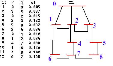
This sample data was taken from Homer Brown's book "Solution of Large Networks by Matrix Methods". The elements of the Zbus matrix can be used to get an equivalent for a subnetwork, thus reduce the amount of input data for subsequent computer runs. If you are performing a study of a distribution network and that network is connected to the substation of a large trasmission grid, you may reduce the large grid into a single impedance to ground if you just want to retain one node. If your distribution network has more than one connections to the large grid, you have to retain those n-connections.
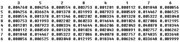
Shown above is the full matrix for the sample data. We want to perform an equivalent for 2 nodes retained. These 2 nodes may be far apart from each other. As shown on the gif file, put the necessary Zij elements, perform an inversion and get an equivalent line impedance.
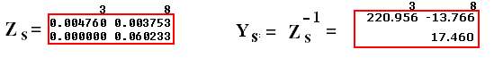
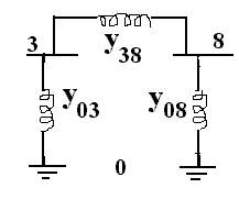 | Zs represents the Zbus of the subnetwork of the figure on the leftside. Ys is its Ybus. By definition, Yii is the sum of node connections and Yij is the negative of ij_admittance. This definition is in Chapter 5. We can therefor get Y[3,8]=-13.766 and y[3,8]=+13.766. We may now solve for y[0,3] and y[0,8].
Y[3,3]=y[0,3]+y[3,8].
y[0,3]=Y[3,3]-y[3,8].
y[0,3]=222.956-13.766=207.18
Also, y[0,8]=17.46-13.766= 3.693
So, z[0,3]=1/y[0,3]=0.00482
z[0,8]=1/y[0,8]=0.2707 and z[3,8]=1/y[3,8]=0.0726
|
The new line data corresponding to the reduced network is
z[0,3]=0.00482, z[0,8]=0.2707 and z[3,8]=0.0726
Using this data, we can form the Zbus again and it will be equal to Zs as shown above. This shows that a large network can be reduced, or a part of a large network can be equivalenced for short circuit computations. As a reminder, we did not show that these numbers are (j) and its reciprocal will have to consider the meaning of (j). You should be concerned about (j) when performing complex numbers later.
4.19 Axes Discarding in Zbus
If the study is on Part B only, the effect of Part A can be included as shown below.
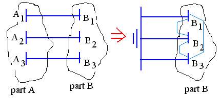
A large set of data for Part A has been reduced to only 6 elements, depending on the number of tie-lines between Parts A and B. Zs is full matrix such that all nodes represented by B1,B2,B3 are connected to one another by an equivalent impedance. Axes refer to the row-column of the Zbus matrix. The use of axes discarding will simplify this procedure. In the formation of the matrix for area B, if the mesh equivalent lines of area A are processed first, the matrix that will result after processing only the equivalent will be exactly Zs. All the steps after the extraction of Zs like
1)inversion of Zs,
2)computing the equivalent lines and
3)forming Zs using these eqivalent lines - - - are unnecessary. All that was accomplished was to collect Zs and move them to the upper left hand corner. The remainder of the matrix was erased.
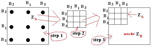
The steps involved in modifying the Zbus matrix to eliminate area A are
1. Zbus (A) with axes of boundary busses indicated
2. The extracted small submatrix
3. Starting point for forming Zbus (B)
As soon as all lines connected to an unwanted bus have been included in Zbus, the row-column of the said bus will never participate in the step-by-step process. Except when a line is included in a coupled group and all members of that group are not yet included in, the row-column is replaced by the last axis. Such process is called "axes discarding". The procedure is depicted below.
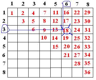
4.20 Half-storage on Zbus in Linear or Vector (array)
Zbus is stored as half triangle because it is symmetrical. Also, it is not stored as square, rather as vector. The sequence is shown on the figure. To access Z[i,j] where i<j, we use the formula:
LOC= I + J*(J-1)/2
As an example, suppose a matrix is 8x8. We would be needing 64 floats or real numbers to store the full matrix. Half storage would require only:
8 + 8*7/2 = 36
Suppose we want Z[3,6],
LOC=3 + 6*5/2 = 18.
|  |
4.21 Axes Discarding on Linear Half Storage
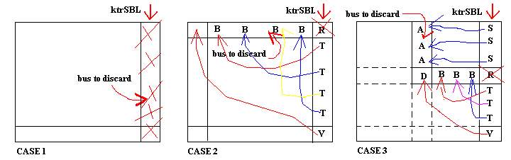
Axis (singular) discarding means that the row-column of the bus to be removed will be replaced by the last column. For Case-1, where the bus is the last bus, simply subtract 1 from the counter SBL (System Bus List). In Case-2, where the bus is the first entry in the matrix, take the diagonal (V) and put it on location=1. Move T's as shown by the arrows. R is discarded. In Case-3, three parts need to be moved. Case-3 will occur if 1<bus<ktrSBL. R is discarded. The sample code fragment below will perform the said movement for all cases.
|
  74: void AxisDiscard(int bus)
  75: {int i,from,to;
  76:  if (bus<ktr_SBL)  //bus, ktr_SBL are subscripts
  77:     {from=LOC[ktr_SBL-1]; to=LOC[bus-1];
  78:      if (bus>1)
  79:          for (i=1; i<bus; i++) X[++to]= X[++from]; //upper
  80:      from++;  //exceed
  81:      for (i=bus+1; i<ktr_SBL; i++)        //lower
  82:        {to=LOC[i-1]+bus; X[to]=X[++from];}
  83:      X[LOC[bus]]=X[LOC[ktr_SBL]];         //diagonal
  84:      from=SBL[bus]; to=SBL[ktr_SBL];      //modify pointers too
  85:      BusPtr[from]=0; BusPtr[to]=bus;
  86:      SBL[bus]=SBL[ktr_SBL];               //busno
  87:     }
  88:   ktr_SBL--;
|
At each step of the Zbus formation, the matrix is printed. Zbus before and after the axis discard is depicted too. Just scroll the text area. Then analyze the program code. Nothing is hidden. Commercial software were based on this technique. It can solve 100 nodes at a time because of matrix size. After solving for fault information, the matrices is rebuilt for the next 100 nodes. If the user specifies which bus need be faulted, then said busses are called "retained" and all others are discarded. There is an exception on this discussion. Other nodes are also retained. They are needed if the fault information is included in NBACK specified by the user(NBACK is the depth of neighborhood). If retained + NBACK are less than 100, then the matrix will be calculated only once.
4.22 Computer Program Discard.C
Quick Win Application has an output that could be cut and paste
to another application. Click edit, then copy after you highlight
some text.
HOME
CHAPTER ONE: INTRODUCTION
CHAPTER TWO: PROGRAMMING TOPICS
CHAPTER THREE: MATRIX INVERSION ROUTINE
CHAPTER FOUR: STEP-BY-STEP ALGORITHMS
CHAPTER FIVE: DIRECT METHODS IN Ybus FORMATION
CHAPTER SIX: SPARSITY
CHAPTER SEVEN: MATRIX FACTORIZATION AND OPTIMAL ORDERING
CHAPTER EIGHT: SPARSE Zbus FROM FACTORED SPARSE Ybus
CHAPTER NINE: FAULT CALCULATIONS
REFERENCES
 --- Eq. (4)
From the matrix equation Z*I=E where only column k of the Zbus is explicitly shown and the current
vector has the single nonzero element
--- Eq. (4)
From the matrix equation Z*I=E where only column k of the Zbus is explicitly shown and the current
vector has the single nonzero element  , the voltages of all the system busses are determined for
unit current injection into bus k.
, the voltages of all the system busses are determined for
unit current injection into bus k.
 is the voltage
across line p-q is,
is the voltage
across line p-q is,