4.1 Step-by-Step Zbus Formation (SSZF)
4.2 Description of the Zbus Matrix
4.3 Description of the SSZF Algorithm
4.4 Type-1 A Branch from the Reference Bus
4.5 Type-2 A Link from the Reference Bus
4.6 Type-3 A Branch not from the Reference Bus
4.7 Type-4 A Link not from the Reference Bus
4.8 Kron Reduction
4.9 Computer Implementation
4.10 Line Reordering Program
4.11 Version1 SSZF Program (ZBUS01.C)
4.12 Mutual Coupling Compensation in (SSZF)
4.13 Type-5 Modified Branch Algorithm
4.14 Type-6 Modified Link Algorithm
4.15 Summary of Formula for SSZF
4.16 Example Calculation SSZF with Mutual Coupling
4.17 Version2 SSZF Program (ZBUS02.C)
4.18 Modified Step-by-Step Zbus Formation
4.19 Modified Step-by-step Ybus Formation
4.20 Example Calculation
4.21 Extension to Large Systems
4.22 Axes Discarding in Zbus
4.23 Zbus Linear Half Storage (LHS)
4.24 Axes Discarding on LHS
4.25 Version3 SSZF with Axes Discarding on LHS (ZBUS03.C)
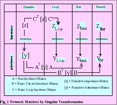
Figure 1 shows the relationship on how we can arrive at one reference using network matrices. We will not study all these matrices. We will concentrate only on those which are important in understanding what the best method is, i.e., computerwise, in solving the short circuit calculation.
The step-by-step Zbus formation will be summarized in this chapter. This topic is still famous because better methods have not been popularized in the academe. Although not practical for large systems, "step-by-step" method can be used easily on software features like line-end fault, sliding fault, and line outage. These options greatly reduces the man-hours required by an engineer in performing fault studies. It also reduces computer time by not rebuilding the sparse Zbus.
4.1 Step-by-step Zbus Formation
his method of finding the inverse of the admittance matrix is done without matrix
inversion . The matrix is built using one element at a time. Theoretical derivation is not included here. The contents of this review is taken from Ref. 9.
4.2 Description of the Zbus Matrix.
The Zbus matrix contains the driving point impedance of every node with respect to
(WRT) a reference bus. The driving point impedance of a node is the equivalent impedance between it and the reference. The off-diagonals are the transfer impedance between each bus of the network and every other bus WRT the reference bus.
The Zbus, also known as "bus impedance matrix" is built from the branch data
consisting of the positive sequence, negative sequence, and the zero sequence impedances. For practical purposes the positive and negative sequence impedances are treated equally.
| 
| 
|
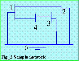
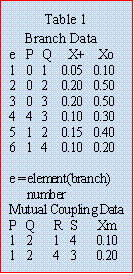
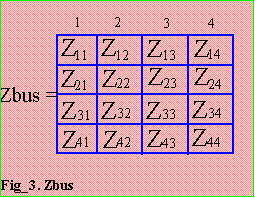
Using the data from Table 1 and sketch shown in Fig_2, the Zbus matrix is shown on Fig_3. During a fault at bus k, all other node currents are neglected, so that for n-node system,
Z * I = E -----Eq. (1.1)
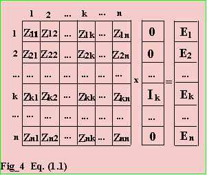
The voltage profile can be determined using column k, provided Ik is known.
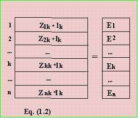
Performing matrix multiplication in Eq. (1.1) yields Eq. (1.2), and all E's are WRT the
Reference Bus.
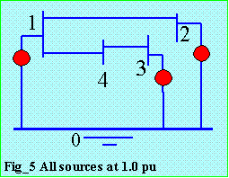
In fault calculations, it is customary to assume that all generators connected to the
network are operating with 1.0 p.u. voltage behind their internal impedance. Please
refer to Fig_5. This common point behind the impedance is used as the reference
node.
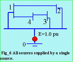
The network can, therefore, be considered to be supplied by a common source. Please refer to Fig_6. The use of 1.0 pu voltage behind the generator impedance can be justified by applying Helmholtz-Thevenin theory. The prefault open circuit voltage at the faulted node is approximately 1.0 pu and may therefore be assumed to be that value. The short circuit impedance of the network from the point of fault is determined by the impedance of the network elements with the internal source voltages all short circuited. The fault current is calculated as superposition of 2 sources:
- the current due to the internal source voltages, which are zero,
- and the current due to a superposed voltage source which will reduce the fault point voltage to zero.
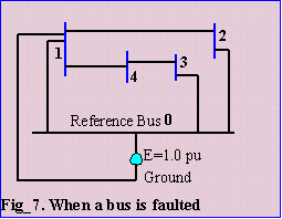
When any node is faulted, it is connected to ground. Full voltage is, therefore, applied between the reference node and the faulted node. For a fault at bus 1, please refer to Fig_7.
Since Zk,k (for k=1,NBUS) are the driving point impedance and the off-diagonals are the transfer impedance WRT the Reference bus, the voltage of Eq_1.1 will all be measured WRT the Reference bus. The Reference bus is, therefore, at zero potential WRT to itself, but is at full voltage WRT the ground. The voltage obtained from Eq_1.1 for the faulted bus is the full voltage of the generators WRT the Reference. In the actual system, the faulted bus is at zero potential WRT the ground. This difference in voltage should cause no difficulty.When any node is faulted, it is connected to ground. Full voltage of 1.0 pu is applied.
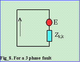

When any node is faulted, it is connected to ground. Full voltage of 1.0 pu is applied.

Eq. (1.3) is for a three phase fault.
From Eq.(1.2), substituting Eq.(1.3) will yield,

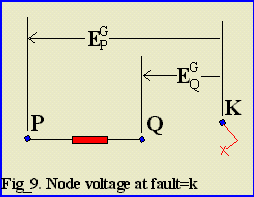
the voltage on bus P WRT the reference for a fault on bus k. The current flow from bus P to bus Q on impedance  is, is,
|
|
 but
but
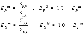
so
 --- Eq. (1.5)
Current flow from bus P to bus Q for a fault at bus k.
The total fault current for a fault on any bus is obtained by Eq. (1.3) and the flow in any branch is obtained by Eq. (1.5). The complete analysis of the system is solved by these simple arithmetic operations once the Zbus matrix has been formed.
4.3 Description of the Step-by-step Zbus Algorithm.
| The system is assembled by starting with a single element connected to the reference bus, adding one element at a time, modifying the matrix for each addition. Each element added should be connected to the system (partial network, PN) by a node (branch) or 2 nodes (link). Element added can be classified into 6 as shown on the right side table. | 
|
4.4 Type-1 A branch from the Reference bus.
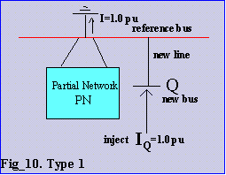
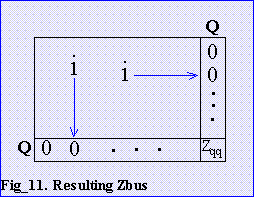
A transformer or generator reactance from the reference to a new bus is identified by finding that one bus is the reference and the other bus is not in the system that has been assembled, the partial network. See Fig_10.
Current of 1.0 pu is injected into the new bus Q which is connected to the Reference, but will produce no voltage on the other busses of PN. Also, injection of current into any bus of PN will produce no voltage on the new bus Q.

The driving point impedance of the new bus is the impedance of the new element added.
For the addition of a branch from the reference to a new bus, augment the Zbus matrix by a row and column of zeroes. The diagonal element of this new axis is the line impedance of the new branch.
4.5 Type-2 A link from the Reference bus.
See Type-4 Equations, Zpi = Zip = 0 , i.e., p=0
4.6 Type-3 A branch not from the Reference bus.
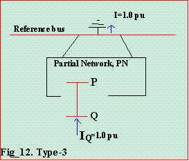
Injecting 1.0 pu current into bus Q is the same as injecting that same current on bus P. Refer to Fig_12.
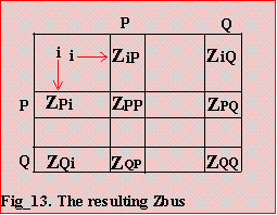
A new axis is added to the Zbus matrix corresponding to the new bus Q. The
off-diagonal elements of the new row-column are the same as the elements of bus P of
the partial network. The diagonal element Zq, where q is obtained as Zp,p + a series line
impedance  .
.

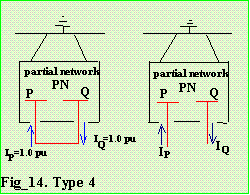
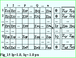
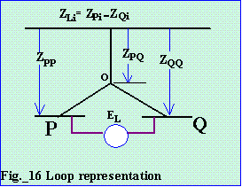
4.7 Type-4 A link not from the Reference bus Adding a link does not introduce a new axis. The response of the partial network to the introduction of a current into the loop created is a constraint that must be satisfied. Injecting 1.0 pu current on bus P causes the voltage to appear at every bus of the partial network that are identical to column P of the matrix. Injecting -1.0 pu current on bus Q produces voltage on the busses of the partial network equal to column Q but opposite in sign. The amount of voltage that must be introduced into the loop to cause a 1.0 pu current in the loop created by addition of a new line.

From Fig_16, segment op is Zpp-Zpq and segment oq is Zqq-Zpq.
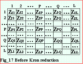

The loop axis is eliminated from the matrix by Kron Reduction. All elements not in the loop row or column are modified. The loop row and column is erased. No new axis is added.
|
4.8 Kron Reduction
In this particular Zbus matrix, it is desired to eliminate the loop row and column. This is equivalent to node elimination by matrix partitioning. Consider Fig_18, where all quantities are submatrices. Solving for | 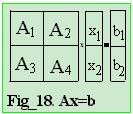
|

and substituting on the first equation yields,

and solving
 ,
,

The coefficient of the unknown
 is seen to be the result of a Kron Reduction when
 is eliminated.
4.9 Computer Implementation
We will start with simple concepts before we tackle difficult
ones. In power systems, a short circuit data file has lines, busses,
and mutual coupling. Lines can mean impedance of transmission line,
transformer, generator, reactor/capacitor, and equivalent circuit
for multi-winding transformers. For simplicity the line data for
our programs on this chapter must be:
contiguous numbering for the busses
no parallel lines
no infinity impedance
no islanding
We do not have a separate bus data since it is not necessary at
this moment. The programs presented will solve x-only and one
sequence network assumed to be the zero sequence. All these
constraints will have to be handled properly later using computing
techniques. Each routine of a program will be thoroughly discussed.
According to increasing sophistication the programs are:
ORDER.C
simple programming RLL (reordered line list) starts from REF
ZBUS_01.C
calls previous ORDER.C full matrix no coupling
ZBUS_02.C
embedded line ordering full matrix, upper triangle only
with mutual coupling
4.10 Line Ordering Program (ORDER.C )
Line ordering is the sequencing of line data so that in the process of step-by-step zbus formation each line added will be connected to the partial network (PN). A line cannot be included into the PN if both nodes are not yet on the PN. System Bus List (SBL) is a the list of busses included on PN. Busses and nodes are synonyms as lines and branches or elements are.
The Zbus building algorithm starts with the Ref on the SBL. During the search on the line data, those connected to Ref will be included on the growing tree. Each line will be added into the PN using types 1,2,3,4 if uncoupled and types 5,6 if coupled. To minimize too much searching on SBL, another vector BusPtr[ ] is used to point to SBL.
The line data maybe traversed several times searching for lines that can be part of a growing tree. It is part of that tree or PN if either its p-side or q-side is already in SBL (including the Reference Bus). Those lines are transferred to RLL. Each node is included to SBL if it was not yet included previously.
Program Listing, Input/Output, just scroll the TextArea.
Some Code Explanation
In this program we just use data index. Later we will use
linked lists . Use of linked
lists will make data index obsolete. There is even no need for this Line Ordering
Algorithm. Line_65 requires us to input from the keyboard the input file. Just uncomment it. Line_69 calls
for the subroutine input() to read the data. The read data is echo printed on the screen.
Program actions are also echo printed. To have a hard copy of program output, just
use file redirection in DOS mode. In Quick Win, highlight the output and click "copy"
and paste it in your Application software.
The data circuit number , positive and zero sequence impedance (or reactance) is not stored in Line_51. Data is terminated by a p-side bus 99, to exit the while (Reading) loop on Line_49. Line data is coded right away to FALSE in Line_55, which means it is not yet reordered. Since it is assumed that bus numbering is sequential, the largest bus number is tracked in Line_56. On exit, we now know nl=line count, and nb=bus count or the largest bus number.
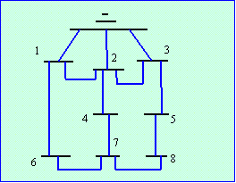
| We start the partial network PN with the Reference bus=0. This is possible in C/C++ because we can access index=0. Old Fortran softwares cannot access index=0 in Line_75. Line_76 is a while loop terminated only if all the lines have been reordered. Be sure to have a correct data, otherwise it might have an infinite loop on this while loop. Another inner loop is a for loop in Line_77 searching for still unordered line, Line_78. In Line_79, the p-side and q-side is taken from the arrays and gets its corresponding address in SBL. If both P and Q are zeroes, it means that the line could not yet be reordered. Skip it for later while loop. |
Line Reordering is needed in the Zbus building Algorithm Version 1. The array RLL[ ] is used to access which line will be added to PN. The data is never really swapped in its address. RLL[ ] is just an index to the data. In section D (supplied by a word processor) is the print for RLL[ ] output. The sequence of lines shows how the partial network will grow. In version 2, we will imbed ordering right in the building of partial network.
Program Listing, Input/Output, just scroll the TextArea.
Some Code Explanation
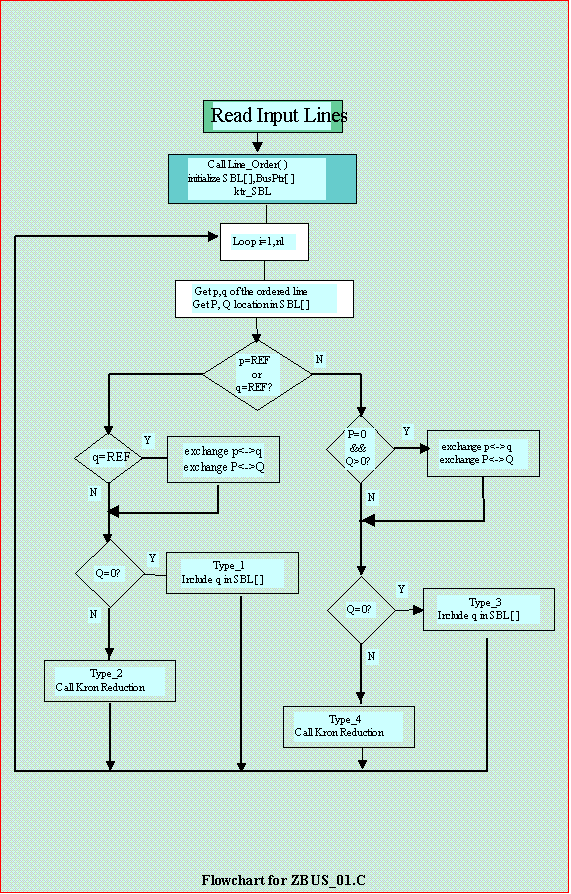
Although this is the simpliest version, count of line codes is 192, quite large for beginners. It is the objective to make programs as simple as possible. There are no error checking for input data validity. These simple programs are not guaranteed bug-free. They are created to implement the previous theories. In this version, we will solve only one sequence Zbus and exclude mutual coupling. Two subroutines-- input( ) and Line_Order( ) are exactly the same as in our program ORDER.C. Lines_24 to _33 are the array/variable definitions. Then we have the subroutine prototypes in Lines_37 to _45. Prototypes can be avoided by placing the main program at the bottom of the listing. There are no type_5 and type_6 subroutines since this will be for our next version.
The main program starts with opening two files. One for reading input data and another for writing output. In Line_171 it is reordered and ready for the growing tree. To do some experimenting, we can sequence the data ourselves and just activate the code in Line_173.
In Line_175 arrays SBL[ ] and BusPtr[ ] are reset to zero as well as the ktr_SBL. Why? ktr_SBL is the size of the partial network. These arrays had been used in reordering. There is no more need for them in the building of the Zbus matrix. We will restart growing the partial network. The ktr_SBL has to start from zero again, that is why it is reset. There is only one sweep for all lines to be processed and complete the Zbus matrix (for loop in Lines_176 to _190). In Line_177 we get the p-side and q-side as well as its location in SBL. You will note that the reference bus=0 is not included in SBL. Type_2 can be executed but it does not mean there are parallel lines from the reference. Parallel lines with mutual coupling is avoided in Step-by-step Zbus formation.
We start the PN with a line fron the reference. Either p or q can be zero. To be in uniformity with our nomenclature we swap p to q if q=0 in Line_182. q must be non-REF. It is q that we add in SBL[ ] for type_1 in Line_65. We do the swapping too for types_3/4 if p is the new bus.
Subroutines type_1/2/3/4 are easily compared with the Summary of Formula on section 4.15.
Program input
The sample input data file here is the same as the data in Table 1 on section 4.2, only that there is a terminator for linedata 99 and terminator for coupling group data 99 and the 98 to mean end of coupling data. We will discuss this coupled group later on. The line data consists of p-side, q-side, circuit number, x-zero sequence, x-positive sequence impedance. You may arrange the sequence in any order and it will be reordered by the subroutine we have developed earlier, the ORDER.C.
Program Output
Output starts with the echo print of the input data read. You will note with the output that there is only one pass and everything had been ordered already. You can try with larger data set. I used smaller data set to highlight only the Zbus formation. We already did the line reordering earlier.
In the matrix printout Before Kron Reduction, you will see the bus header 0. This should be "L" on our paper and pencil example. The computer output here is similar to our example in section 5.4. This one however is more simple because it does not have mutual coupling. We would like to present the programming concepts in less shocking steps.
Further Research: Determine the reason why coupled parallel
lines is prohibited in step-by-step Zbus algorithm.
Chapter 4 continuation.
HOME
CHAPTER ONE: INTRODUCTION
CHAPTER TWO: PROGRAMMING TOPICS
CHAPTER THREE: MATRIX INVERSION ROUTINE
CHAPTER FOUR: STEP-BY-STEP ALGORITHMS
CHAPTER FOUR: Part 2
CHAPTER FIVE: DIRECT METHODS IN Ybus FORMATION
CHAPTER SIX: SPARSITY
CHAPTER SEVEN: MATRIX FACTORIZATION AND OPTIMAL ORDERING
CHAPTER EIGHT: SPARSE Zbus FROM FACTORED SPARSE Ybus
CHAPTER NINE: FAULT CALCULATIONS
REFERENCES
