7.1 Triangularization of a Matrix
7.1 Triangularization of Matrix
7.2 Ordinary LU Factorization
7.3 LU-Dolittle Method (LUDM) for Sparse Matrix
7.4 Code Fragments on LUDM
7.5 Example Calculation
7.6 Optimal Ordering (OO)
7.7 OO Scheme_123 Computer Program (SCHEME123.C)
Triangularization is the process of applying Gauss-Jordan Reduction to solve the simultaneous linear equation of the form Ax=b. LU Factorization where L="Lower" and U="Upper" is synonymous to triangularization. Factorization simply means that when we multiply matrices L and U, we get matrix A. Given the LU, we can perform forward course and backward course on b to solve for x. This is needed in Loadflow calculation. With LU we can also get the inverse of A which is used in short circuit calculation. Factorization is used to solve large sparse matrix A. Sparse means that more A(i,j) elements are zeroes than are non-zeroes. For power systems, it can be just 2 per cent of the square matrix A is non-zero. There are many references on LU Factorization that exploits matrix sparsity. Ref [21] contains clear formula derivation.
7.2 Ordinary LU Factorization
We can derive the formula in LU factorization using a 4x4 size matrix.
The problem can be formulated as:
Given matrix A, solve the elements in matrices
L and U such that L*U = A,
where matrices L and U are factors of A.
Once the elements in L and U are solved,
unknown vector x in the equation A*x = b
can be determined by forward course and
backward course using L and U
. There are variations to the structure of L and U and
other References call these LDU. We choose our form as shown below.
 --- Eq. (1)
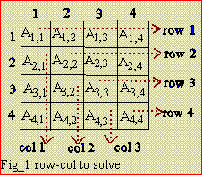
Performing matrix multiplication, each A(i,j) elements can be equated as product of a row of L and a column of U. Remember that matrix A is know quantity and matrices L and U are unknown factors of A.
|
Row=1. Equating elements on row=1 as shown by the dotted
arrow. These elements are A(1,1), A(1,2), A(1,3), A(1,4):
A(1,1)=1*U(1,1); A(1,2)=1*U(1,2); A(1,3)=1*U(1,3);
Col=1. Equating elements on col=1, these are A(2,1), A(3,1),
A(4,1):
|
|
At this stage, U(1,1) had been solved already. So
L(2,1)=A(2,1)/U(1,1)
L(3,1)=A(3,1)/U(1,1)
L(4,1)=A(4,1)/U(1,1)
Row=2. Equating elements A(2,2), A(2,3), A(2,4):
A(2,2)=L(2,1)*U(1,2) + 1*U(2,2)
so U(2,2)=A(2,2) - L(2,1)*U(1,2)
where L(2,1) and U(1,2) had been previously solved.
Also,
A(2,3)=L(2,1)*U(1,3) + 1*U(2,3),
so U(2,3)=A(2,3) - L(2,1)*U(1,3), where U(1,3) was previously solved.
A(2,4)=L(2,1) - U(1,4) + 1*U(2,4),
so U(2,4)=A(2,4) - L(2,1)*U(1,4), where U(1,4) was previously solved.
Col=2. Equating elements A(3,2), A(4,2):
A(3,2)=L(3,1)*U(1,2) + L(3,2)*U(2,2)
so L(3,2)=(A(3,2) - L(3,1)*U(1,2))/U(2,2) where necessary right hand terms were previously solved.
A(4,2)=L(4,1)*U(1,2) + L(4,2)*U(2,2)
L(4,2)=(A(4,2) - L(4,1)*U(1,2))/U(2,2)
Row=3. Equating elements A(3,3), A(3,4):
A(3,3)=L(3,1)*U(1,3) + L(3,2)*U(2,3) + 1*U(3,3)
The unknown here is U(3,3).
U(3,3)=A(3,3) - L(3,1)*U(1,3) - L(3,2)*U(2,3)
A(3,4)=L(3,1)*U(1,4) + L(3,2)*U(2,4) + U(3,4)
U(3,4)=A(3,4) - L(3,1)*U(1,4) - L(3,2)*U(2,4)
Col=3. Equating elements A(4,3):
A(4,3)=L(4,1)*U(1,3) + L(4,2)*U(2,3) + L(4,3)*U(3,3)
L(4,3)=(A(4,3) - L(4,1)*U(1,3) - L(4,2)*U(2,3))/U(3,3)
For ordinary LU, we can generalize that for matrix of size N,
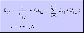 --- Eq. (2) --- Eq. (2)
Equating elements A(4,4): A(4,4)=L(4,1)*U(1,4) + L(4,2)*U(2,4) +L(4,3)*U(3,4) + U(4,4) U(4,4)=A(4,4) - L(4,1)*U(1,4) - L(4,2)*U(2,4) - L(4,3)*U(3,4) And also , | 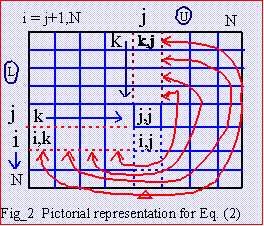
|
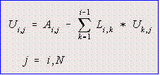 --- Eq. (3) --- Eq. (3)
By looking at Eqs (2) and (3), we can conclude that there is no need to store L,U and A as three matrices. Use only one matrix A. After the factorization, matrix A is destroyed and replaced with L and U. The diagonal of matrix L is not stored. To do: Write a computer program to perform Ordinary LU Factorization using only one matrix. | 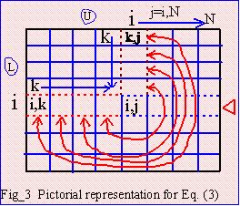
|
7.3 LU-Dolittle Method (LUDM) for Sparse Matrix.
|
This factorization is applicable for sparse matrices with
half-storage. After solving for row 1 and col 1, modify those
inside the enclosed dotted square (or rectangle),
Loop 1: A'(2,2) = A(2,2) - L(2,1)*U(1,2), A'(2,3) = A(2,3) - L(2,1)*U(1,3), A'(2,4) = A(2,4) - L(2,1)*U(1,4), A'(3,2) = A(3,2) - L(3,1)*U(1,2), A'(3,3) = A(3,3) - L(3,1)*U(1,3), A'(3,4) = A(3,4) - L(3,1)*U(1,4), A'(4,2) = A(4,2) - L(4,1)*U(1,2), A'(4,3) = A(4,3) - L(4,1)*U(1,3), A'(4,4) = A(4,4) - L(4,1)*U(1,4). | 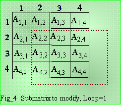
|
Where U(2,2) = A'(2,2), U(2,3) = A'(2,3), and U(2,4) = A'(2,4)
Also L(3,2) = A'(3,2)/U(2,2) and L(4,2) = A'(4,2)/U(2,2)
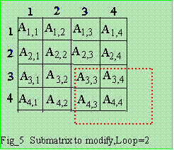
Loop 2 :
|
A"(3,3) = A'(3,3) - L(3,2)*U(2,3),
A"(3,4) = A'(3,4) - L(3,2)*U(2,4), A"(4,3) = A'(4,3) - L(4,2)*U(2,3), A"(4,4) = A'(4,4) - L(4,2)*U(2,4).
Where U(3,3) = A"(3,3) , U(3,4) = A"(3,4)
| 
|
For symmetric matrix there is no need of saving matrix L.
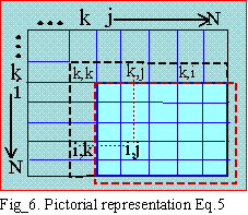
In program implementation we make a k-loop
from 1 to N-1. As shown on Fig_6 on the k_th loop, we need to
update A(i,j)'s inside the big red dotted square (for colored print).
To solve a particular A(i,j), we
need L(i,k) and U(k,j) pointed to by the small dotted red line.
However L(i,k)=U(k,i)/U(k,k), so to save memory there is no need
to store matrix L because its value can be derived from U itself. For
half-storage, storing only U, then,
 --- Eq. (4) --- Eq. (4)
| 
|

 --- Eq. (5)
| The original matrix [A] is destroyed. Resulting [U] is stored on [A] itself, so only one matrix is used. This is similar to Shipley inversion. By looking at Eq. (5) and Fig_7, we are now on loop=k and the rectangles represents rhs nodes of k. There are 4 here and by Eq. (5) we must modify 4 diagonal elements and 6 off-diagonals, ij, y1,y2,y3,y4, and y5 as we modify only the upper triangle. If location represented by ij is not in lifo then it is a fill-in. The purpose of Node Ordering is to minimize (not really absolute minimum) the total fill-ins introduced during the factorization. | 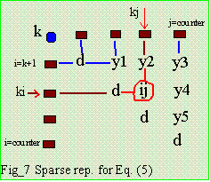
|
7.4 Code Fragments on LUDM
code=1: LUDM factorization Full Matrix, Upper Triangle only

1: for (k=1;k< nb;k++)
2:   for(i=k+1;i<= nb;i++)
3:     for (j=i;j<= nb;j++)   <- note j=i
4:        Y[i][j]-=Y[k][i]*Y[k][j]/Y[k][k];

code=2: Full matrix, Simulates sparse code

1:   for (k=1;k< nb;k++)
2:      for(i=k+1;i<= nb;i++)
3:         {Y[i][i]-=Y[k][i]*Y[k][i]/Y[k][k];
4:            for (j=i+1;j<= nb;j++)                <- note j=i+1
5:               Y[i][j]-=Y[k][i]*Y[k][j]/Y[k][k];
6:         }

code=3: LUDM Factorization of Sparse Ybus,Compact Numbers,Without Ordering

1: void Factor(void)
2: {int kk,i,j,ij,ki,kj,I,J,EndBus[20],Adr[20],counter;
3: /*All matrices had been reset (=zero) at Ybus()*/
4:  for (kk=1;kk< nb;kk++)
5:      {counter=Get_RHSnodes(kk,EndBus,Adr);   //number of RHS elements
6:        if (counter)    /*perform finite change on upper triangle only*/
7:            for (i=1;i<= counter;i++)
8:                {I=EndBus[i];ki=Adr[i];
9:                 YPd[I]-=YP[ki]*YP[ki]/YPd[kk];       // Diagonal part
10:               if (i< counter)
11:                   for (j=i+1;j<= counter;j++)       // Off-diagonal part
12:                        {J=EndBus[j];kj=Adr[j];
13:                          ij=BrnSrNsrt(I,J);        //branch search-insert J
14:                          YP[ij]-=YP[kj]*YP[ki]/YPd[kk];
15:                         } /*for j*/
16:                  }  /*for i*/
17:     }  /*for kk*/
18: }

code=4: LUDM Factorization of Sparse Ybus,Non-compact Numbers,With Ordering

1: void Factor(void)
2: {int k,kk,i,j,ij,ki,kj,I,J,EndBus[20],Adr[20],counter;
3:   for (k=1;k< nb;k++)
4:       {kk=NewOrder[k];
5:         counter=Get_RHSnodes(kk,EndBus,Adr);
6:         if (counter)   //perform finite change on upper triangle only
7:            for (i=1;i<= counter;i++)
8:               {I=EndBus[i];ki=Adr[i];
9:                YPd[BusPtr[I]]-=YP[ki]*YP[ki]/YPd[kk]; //Diagonal part
10:              if (i< counter)
11:                  for (j=i+1;j<= counter;j++)       //Off-diagonal part
12:                    {J=EndBus[j];kj=Adr[j];
13:                     ij=BrnSrNsrt(I,J);   //branch search-insert I->J
14:                     YP[ij]-=YP[kj]*YP[ki]/YPd[kk];
15:                     } /*for j*/
16:              }  /*for i*/
17:       }  /*for k*/
18: }
|
Explanation of codes.
Both codes=1 and 2 are implemented in full matrix notation, but computation is done only on the upper trangle. In code=1 the line Y[i][j]-=Y[k][i]*Y[k][j]/Y[k][k]; should have been Yij = Yij - Yik*Ykj/Ykk if the lower part was also solved. But since only the upper triangle was solved and we do not store the L matrix, Yki is used instead of Yik because k is less than i and also k is less than j. Note that the third loop starts at j=i, while code=2 has j starts at j=i+1. In code=1, when i=k+1 and j=i (j=k+1) represents that the Yij being updated is the diagonal or Yii. It is thus equal to Yii-=Yki*Yki/Ykk. For code=2 and 3,the update of the diagonal must be separate from the update of the off diagonal, because the diagonal is saved in a different memory location, i.e. code=2 is a full matrix that simulates code=3. We can do this by having j=i+1. Before going to the j-loop, the diagonal Yii must have been updated first.
In code=3, the End nodes of k are stored in EndBus[] and its address is stored in Adr[] starting from 1 to counter. Only RHS nodes are stored with or without ordering scheme. The j-loop starts from j=i+1 similar to code=2. Prior to j-loop, the diagonal Yii which is stored in a separate vector, Ypd[I], where I is the end node. The off diagonal Yij is computed as; YP[ij]-=YP[kj]*YP[ki]/YPd[kk];
where kj and ki are addresses stored in Adr[], while ij is searched in lifo. If absent, this becomes a fill.
When i=counter, there is no more off diagonals to be solved.
Thats why a test "if (i The call to "Get_RHSnodes(kk,EndBus,Adr)" for code=3 and code=4
are the same. "kk" in code=4 is also a compact number.
7.5 Example Calculation.
7.6 Optimal Ordering.
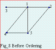
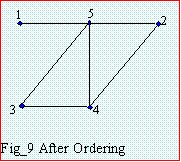
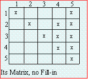
When the matrix to be factored is sparse, the order in which rows are processed affects the number of
fill-ins. If the order (or bus numbering) is shown as in Fig_8, there will be 4 fill-ins. If however, the node with
most connections is numbered last, corresponding factorization will insert no fills as shown in Fig_9. Great
savings in arithmetic operations and computer storage can be achieved if we can minimize the fill-ins
introduced, particularly in repeat solutions as in Fast Decoupled Loadflow. Repeat solution means that the
factored matrix remains the same for several iterations. Tinney-Walker [19] discusses optimal ordering known
as schemes 1,2 and 3. The program implementation may not be exactly as described in Ref. 19.
Scheme 2
1. Nodes with valence=1 are renumbered rightaway.
7.7 OO Scheme_123 Computer Program (SCHEM123.C)
Factored Ybus=
1 2
3
4
1 36.6667 -6.6667
0 -10.0
2 10.4545 0
-1.81818 *
3 15.0 -10.0 4 10.2899
* where Y2,4 is a fill-in.
Scheme 1
Number the rows according to the number of nonzero off-diagonal terms before the factorization. When fill-ins are added to the sparse matrix after factorization, the off-diagonal terms would increase. In this scheme the rows with only one off-diagonal term are numbered first sequentially from index 1 to bus count, those with two terms, etc., and those with the most terms, last. This scheme does not take into account any of the subsequent effects of the process. The only information needed is a list of the number of nonzero terms in each row (or off-diagonals) of the original matrix(i.e. unfactored). The second version uses a little technique to speed up ordering.
Number the rows so that at each of the process the next row to be operated upon is the one with the fewest nonzero terms. If more than one row meets this criterion, select any one. This scheme requires insertion of fills in the process as the bus is ordered. Subtract one from NumOffDiag[ ] to all its rhs nodes and add one for nodes k-m (the fill-in). Increase valence counter until all the nodes are ordered.
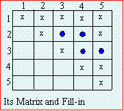
Scheme 3
Number the rows so that at each step of the process the next row to be operated upon is the one that will introduce the fewest fill-in. We can speed up computer time by simulating factorization and process busses that have rhs nodes=valence count and order the busses starting from minimum fill. As the bus is ordered insert its fill and subtract one from NumOffDiag[ ] to all its rhs nodes and add one for nodes k-m (the fill-in).
Repeat the loop since other NumOffDiag[ ] had changed until no nodes are ordered. This time increase valence counter until all the nodes are processed. Scheme-3 is implemented as,
2. Compute table of fills for unrenumbered nodes, only for valence<=k.
3. The next node to be renumbered is the node with minimum fill, (say fill=1).
Renumber all nodes as determined in (2) starting from minimum fill, insert the fill.
4. Loop back to 2. This looping will take several times as other nodes have NumOffDiag[ ]
becoming =valens.
5. increase valence count and Loop back to 2 until all nodes are renumbered
In application programs such as loadflow and short circuit, the
user must have an option to choose between schemes. However,in short
circuit there is no such thing as repeat solution compared to loadflow.
Question: How do you know that a branch is a fill-in or an impedance?
Answer: A branch is a fill-in if its address is above 1->LINES. All fill-ins are appended after address LINES.
Observation: Scheme 2 and 3 simulates LU factorization.
Fill-ins are inserted. So during actual LU factorization, there is no
need to insert fil-ins,otherwise there is a bug in the program.
Further Research: Dynamic programming can be applied to scheme 3.
The choice which node will be renumbered next should contribute minimum fill.
All the paths taken should arrive at a global minimum.
HOME
CHAPTER ONE: INTRODUCTION
CHAPTER TWO: PROGRAMMING TOPICS
CHAPTER THREE: MATRIX INVERSION ROUTINE
CHAPTER FOUR: STEP-BY-STEP ALGORITHMS
CHAPTER FOUR: Part 2
CHAPTER FIVE: DIRECT METHODS IN Ybus FORMATION
CHAPTER SIX: SPARSITY
CHAPTER SEVEN: MATRIX FACTORIZATION AND OPTIMAL ORDERING
CHAPTER EIGHT: SPARSE Zbus FROM FACTORED SPARSE Ybus
CHAPTER NINE: FAULT CALCULATIONS
REFERENCES
Copyright © 1997 by Sparsity Technology. All rights reserved.
