5.1 Positive Sequence Ybus Formation
5.1 The Method of Singular Transformation (MST)
5.2 Example Calculation
5.3 Computer Technique for MST
5.4 Example Calculation, Direct Method, K.Nagappan Style
5.5 Another Computer Technique for MST, Direct Method
5.6 Matrix Multiplication, MST Program (SINGULAR.C)
5.7 Computer Program for Direct Method (DIRECT.C)
5.8 Positive Sequence Ybus Formation
5.9 Example Calculation
5.10 Treatment of Parallel lines with Coupling
5.11 Processing Coupling on a per Group Basis
The Ybus formation for short circuit in the positive sequence is similar as that used in loadflow. Line charging, off-nominal transformer tap, reactive shunts are included unlike in step-by-step Zbus where all these are neglected to simplify the computing procedure. Accuracy can be further increased by treating loads as constant impedance/admittance, just like in transient stability and Zbus loadflow. Converged bus volatge can be used in fault calculation instead of just 1.0 pu.
1) The constant admittance load at bus i is
 where is the converged loadflow voltage
= g - jb for inductive load
|
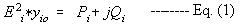
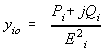
2) The equations for an off-nominal tap transformer in equivalent pi is
| 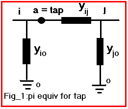
|
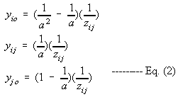
 =transformer impedance,
 =resulting shunts
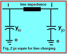
3) Transmission line charging is
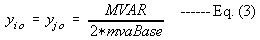
MVAR= total line charging mvaBASE= 100 mva base The 2 in the denominator of Eq. (3) simply means that the Mvar charging is equally divided as in pi-model. When Mvar is divided by Base, it results to pu admittance. 4) Reactive shunt is
| 
|
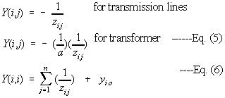
the second part of Eq. (6) is due to load, transformer shunt or line charging. It is also a summation if there are more of them. Eqs. 5 and 6 constitute to what is referred to as nodal admittance matrix. The matrix formed is called as Ybus.
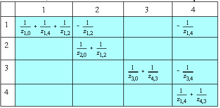
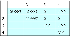
5.2 Example Calculation.
The data is from section 4.2.
The off-diagonal elements are;
Ybus is symmetric. Plugging the computed elements in matrix,
5.3 The Method of Singular Transformation (MST)
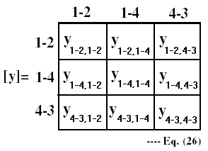
Ybus with coupling can be solved using Singular Transformation, see Ref 2. First we define some variables and terms. Branch and link are terminologies in graph theory.
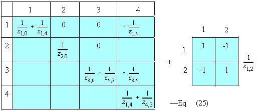
Example Formation of  and A
We can visualize better how each element of the coupling matrix [z] affects
Y(i,j) by considering the Ybus of Eq. (7) when line 1-2 is taken out of the
matrix. The said z(1,2) here is the self impedance and the matrix does not contain
mutual coupling. The figure below is not a real matrix addition as it must be
compatible in matrix size. The figure is just a visual representation of how to
include the effect of z(1,2) inside the Ybus matrix. By the figure, it says that
z(1,2) is added to 4 elements -- Y(1,1), Y(1,2), Y(2,1), and Y(2,2) and taking care of
whether it is positive or negative as shown by 1 or -1 inside the 2x2 matrix.
The programming logic then becomes;
Search the entire [y] and update 4 elements. We can not just search the
upper triangle of [y] to perform the update because by inspection: Y(1,1) has the
elements y(1-2,1-4) and y(1-4,1-2), also Y(4,4) has y(1-4,4-3) and y(4-3,1-4).
So search the entire [y]. To implement this procedure for the upper triangle
portion of Y(), see to it that the 4 elemnets Y(i,j) solved has P<=Q, P<=S,
Q<=R and Q<=S and use all elements of [y]. This method is also true for
sparse matrix application. Note that for sparse matrix, only the upper
triangle is stored and P,Q OR Q,P can be accessed using start[P] or start[Q].
When the program uses node ordering, upper triangle is based on this node
ordering. See the topic when a node is left-side or right-side of a diagonal.
Some Code Explanation
This program could not be used for large data because of matrices involved. This
is created only to check the validity of the next computer technique, the Direct
Method. The Bus incidence matrix A is formed rightaway while reading the line data
in line_123. The diagonal of the primitive impedance matrix [z] is also formed. While
reading the coupling data on line_128, the off-diagonal of [z] is also filled up in
lines_133 to 137. Proper sign or direction of coupling is taken cared of depending
its entry in pq-rs vectors. The matrix At[][] is used to store the transpose of A
in line_154 of the main program. In line_159, Shipley is called to invert [z]. Only
one matrix is used as this is an in-place inversion. The product At*[y] is stored in
Ytemp[][] in line_166. The final product is done in line_172 and Ybus is stored in Y[][].
Program Code for MST, Full Matrix, Upper Triangle only
 --- Eq. (7)
The diagonal elements are;
Y(1,1)=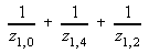 = 1/0.05 + 1/0.10 + 1/0.15 = 36.666
Y(2,2)= = 1/0.2 + 1/0.15 = 11.667
Y(3,3)= = 1/0.2 + 1/0.10 = 15.0
Y(4,4)= = 1/0.10 + 1/0.10 = 20.0
Y(1,2)= = - 1/0.15 = -6.667
Y(3,4)= = - 1/0.10 = -10.0,
Y(1,4)= = - 1/0.10 = -10.0
 has a(i,j)= 1 if ith element is incident to and oriented away from jth node.
1. n, nodes= or busses, junction of one or more elements. Reference bus is designated as node=0.
2. e, elements=lines, transformer or generator impedance or its equivalent circuits. Synonymous to branches in other topics, except here.
3. branch= element when added to the partial network does not close a loop
4. link= element when added to the partial network closes a loop
5. Partial Network (PN)=a connected graph of a network. All elements are not yet included.
6. Â= element-node incidence matrix, shows the incidence of elements in a connected network.
= -1 if ith element is incident to and oriented from jth node.
= 0 if not incident to jth node.
The definition above requires a direction of elements. It is similar to the definition in powerflow that a MW flow on a line away from a node is + and if towards the node -. For simplicity a(i,j)=1 for a "From Bus", and a(i,j)= -1 for a "To Bus". Here, the direction is dictated by p-q entry in the input data.
 = Element-node Incidence Matrix, and A= Bus Incidence Matrix
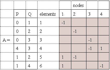
See Table 1 and Fig_1 on section 4.2 for the data used in this section.
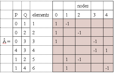
When the reference bus 0 is deleted from the  (element-node incidence matrix whose size is row=6, columns=5), it becomes A (bus incidence matrix whose
size is row=6, columns=4). Note that element 4-3 is in conformity with
the coupling data. The from bus here is 4 (positive) and the
to bus is negative. The shaded portion is the actual matrix.
The A (bus incidence matrix) is shown below.

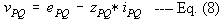
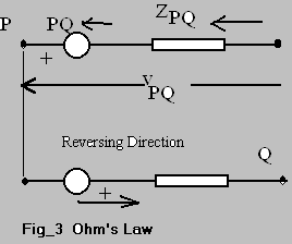
From Ohm's Law, the drawing on Fig_3 v=E-z*I
Reversing the directions, in impedance form,
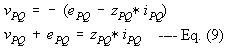
In admittance form, dividing Eq. (9) by zPQ
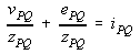
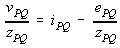
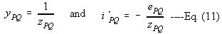
 and also from Eq. (9)
A set of unconnected elements is defined as primitive network. The
performance equation of a primitive network can be derived from Eqs. (12)
and (13) by expressing
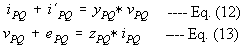
[i] + [i'] = [y][v] admittance form --- Eq. (14)
[v] + [e] = [z][i] impedance form --- Eq. (15)
where [i] = all branch currents, including sources
[z], [y] = are primitive impedance and admittance.
z[i,i]= diagonal, is the self impedance
z[i][j]= off-diagonal, is the mutual impedance of
element i to element j.
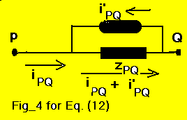
Pre-multiply Eq. (14) by

where [A] is the bus incidence matrix.
But , because of Kirchauff's Current
Law, "The algebraic sum of currents in a bus is zero."
, because of Kirchauff's Current
Law, "The algebraic sum of currents in a bus is zero."
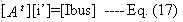
Eq. (17) refers to the algebraic sum of source currents at a bus, which
is the injected current. From Eq. (16)

By power-invariant rule, the sum of powers in the primitive network
is equal to the sum of powers in the interconnected network.
From Eq. (19) we need to take the conjugate (*) of [Ibus] then get its
transposed. Using Eq. (17);
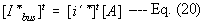
Eq. (20) is so because
Substituting Eq. (20) in Eq. (19)

Substitute Eq. (21) in Eq. (18) for [v];
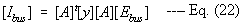
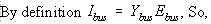
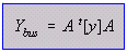 --- Eq. (23)
5.7 Another Computer Technique to MST, Direct Method
 --- Eq. (25)
Shown below is the [y] and by observation, each element in [y]
affects 4 elements in Ybus. This is similar to the figure in Eq. (25). This
observation can improve steps 5,6, and 7 of section 5.5. As an example,
y(1-2,4-3) will affect the following
1) Y(1,4) += y(1-2, 4-3)
2) Y(1,3) -= y(1-2, 4-3)
3) Y(2,4) -= y(1-2, 4-3)
4) Y(2,3) += y(1-2, 4-3)
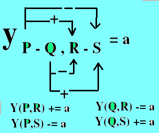
When all the elements of [y] are taken outside the Ybus, the figure below
shows how each element can be added to the matrix. This has a good analogy to
Eq. (25).
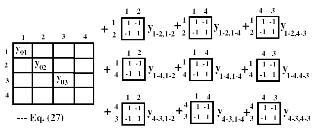
1. Build partial Ybus, those branches not included in a
   coupling group. The first matrix in Eq. (27).
2. Loop for all coupled groups.
3.    Form the primitive impedance matrix [z]
4.    Invert [z] to get [y] using Shipley Inversion
5.    Each y(p-q,r-s) of [y] affects 4 Y(i,j)'s of Ybus.
      Perform the add/subtract.
6. Next coupled group.
Code Snippet for Full Matrix with upper triangle update only

for (i=1; i< z_size; i++)
  {lp = zP[i]; lq = zQ[i];
   for (j=1; j<= z_size; j++)
      {lr = zP[i]; ls = zQ[j];  //there is no zR[ ], zS[ ] here
       if (lp<=lr)  YZ[lp][lq] += cmat[i][j];
       if (lp<=ls)  YZ[lp][ls] -= cmat[i][j];
       if (lq<=lr)  YZ[lq][lr] -= cmat[i][j];
       if (lq<=ls)  YZ[lq][ls] += cmat[i][j];
      }
   }

Code Snippet for Sparse Matrix without Node Ordering

     Y(p,r)=Y(p,r) + y(pq,rs)   Y(p,s)=Y(p,s) - y(pq,rs)
              ^ ^      ^  ^              ^ ^      ^   ^
     Y(q,r)=Y(q,r) - y(pq,rs)   Y(q,s)=Y(q,s) + y(pq,rs)
              ^ ^       ^ ^              ^ ^       ^  ^
for (i=1; i< z_size; i++)
  {lp = zP[i]; lq = zQ[i];
   for (j=1; j<= z_size; j++)
      {lr = zP[i]; ls = zQ[j];
       if (lp==lr) YZd[lp] += cmat[i][j];   //diagonal
         else if (lp< lr)  YZ[BrnSrNsrt(lp,lr)] += cmat[i][j];
       if (lp==ls) YZd[lp] += cmat[i][j];   //diagonal
         else if (lp< ls)  YZ[BrnSrNsrt(lp,ls)] += cmat[i][j];
       if (lq==lr) YZd[lq] += cmat[i][j];   //diagonal
         else if (lq< lr)  YZ[BrnSrNsrt(lq,lr)] += cmat[i][j];
       if (lq==ls) YZd[lq] += cmat[i][j];   //diagonal
         else if (lq< ls)  YZ[BrnSrNsrt(lq,ls)] += cmat[i][j];
      }
   }
Program code for Singular Transformation
HOME
CHAPTER ONE: INTRODUCTION
CHAPTER TWO: PROGRAMMING TOPICS
CHAPTER THREE: MATRIX INVERSION ROUTINE
CHAPTER FOUR: STEP-BY-STEP ALGORITHMS
CHAPTER FOUR: Part 2
CHAPTER FIVE: DIRECT METHODS IN Ybus FORMATION
CHAPTER SIX: SPARSITY
CHAPTER SEVEN: MATRIX FACTORIZATION AND OPTIMAL ORDERING
CHAPTER EIGHT: SPARSE Zbus FROM FACTORED SPARSE Ybus
CHAPTER NINE: FAULT CALCULATIONS
REFERENCES
